QC and Sample Size Estimation

Purpose

This vignette demonstrates how the package can be used to create descriptive statistics or quality control plots for a dataset. First, we read a “proteinGroups.txt” file from the MaxQuant software, and next, we specify a prolfqua configuration. Afterward, the data is transformed and normalized, and plots describing the data are generated. Finally, we estimate how many samples are necessary to properly quantify a two-fold change for \(90%\) of all the proteins with a power of \(0.8\).

Loading data

Generate Simulated data. To learn how to create prolfqua LFQData objects see the vignette: creating configurations.

simdata <- prolfqua::sim_lfq_data_peptide_config()
lfqdata <- prolfqua::LFQData$new(simdata$data,simdata$config)
lfqdata$remove_small_intensities()

You can convert the data into a data frame in a wide format, where the intensities of each sample occupy their columns.

lfqdata$to_wide()$data[1:3,1:8]

## # A tibble: 3 × 8
##   protein_Id  peptide_Id isotopeLabel  A_V1  A_V2  A_V3  A_V4  B_V1
##   <chr>       <chr>      <chr>        <dbl> <dbl> <dbl> <dbl> <dbl>
## 1 0EfVhX~0087 ahQLlQY7   light         26.9  25.2  26.1  25.2  26.1
## 2 0EfVhX~0087 dJkdz7so   light         NA    16.1  14.7  NA    25.7
## 3 0EfVhX~0087 ITLb4x1q   light         19.4  NA    18.2  18.9  28.9

Visualization of not normalized data

Next we show how the data is distributed before transformation and normalization.

lfqplotter <- lfqdata$get_Plotter()
lfqplotter$intensity_distribution_density()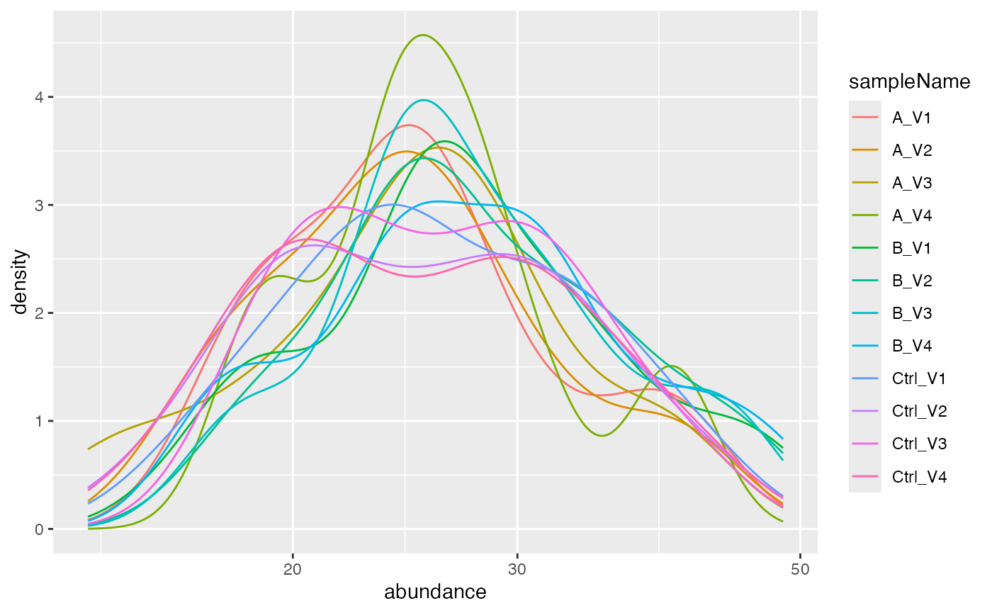

Visualization of missing data

Often it also makes sense to look into the part of the data that is not quantified in all samples. Therefore several functions for the missingess are available. In the NA_heatmap function it is possible to see if some missing proteins are specific for one particular dilution or if they appear randomly in all samples.

nah <- lfqplotter$NA_heatmap()

Prints missing heatmap:

nah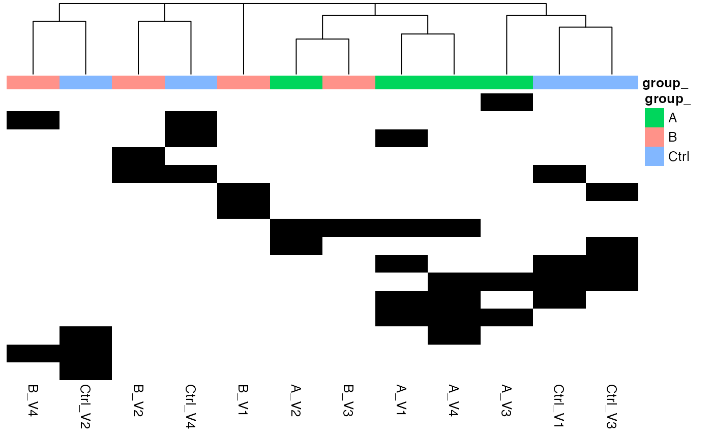

Heatmap, black - missing protein intensities, white - present

Also in the next two figures we show how many missing values are found in the respective conditions and how many proteins do not have missing data and how complete the measurements are for each group.

lfqdata$get_Summariser()$plot_missingness_per_group()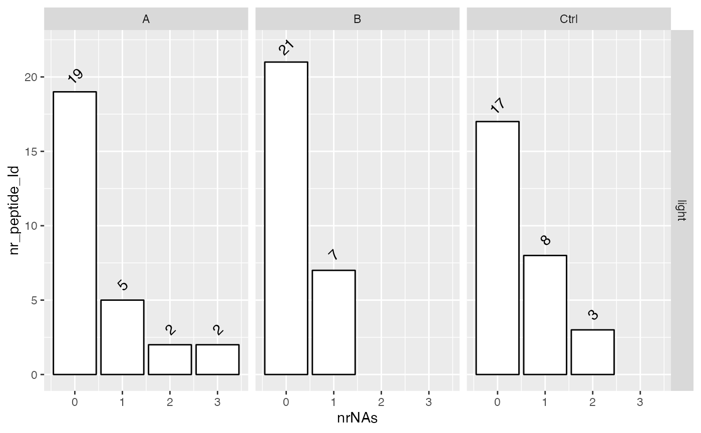

# of proteins with 0,1,…N missing values

lfqdata$get_Summariser()$plot_missingness_per_group_cumsum()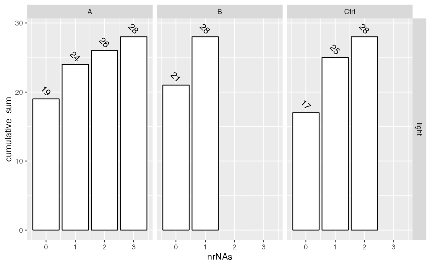

Cumulative sum of the # of proteins with 0,1,…N missing values

In the missigness_histogram we can check if there is a dependency between NAs (and the number of NAs for earch protein) with respect to the protein intensity.

lfqplotter$missigness_histogram()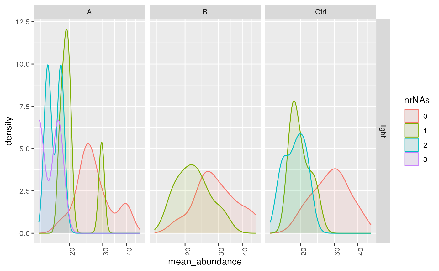

Intensity distribution of proteins depending on # of missing values

Computing standard deviations, mean and CV.

Other important statistics that can be easily calculated from the object are coefficient of variation, means and standard deviations.

stats <- lfqdata$get_Stats()

## [1] "group_"
## NULL

prolfqua::table_facade( stats$stats_quantiles()$wide, paste0("quantile of ",stats$stat ))

quantile of CV
probs	A	All	B	Ctrl
0.10	1.215060	7.185163	1.236542	1.129780
0.25	2.442726	12.277918	1.999453	1.607515
0.50	3.418211	15.169313	3.026062	3.349758
0.75	4.599101	19.467593	4.155821	4.885600
0.90	6.349093	21.451325	5.322302	6.008022

stats$density_median()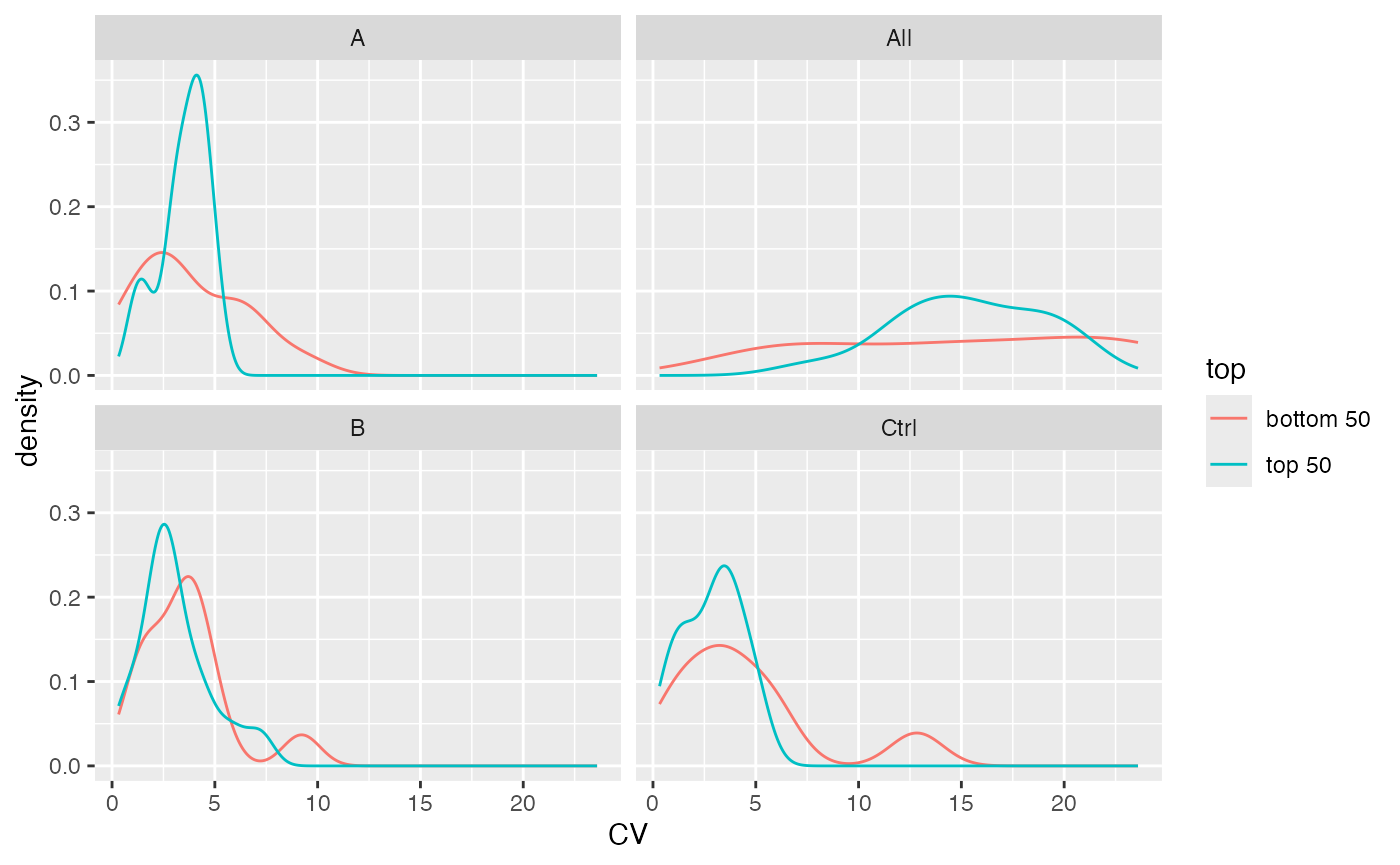

Distribution of CV’s

In the next figure we show the dependency of the standard deviation with respect to the mean intensitiy of the proteins.

stdm_raw <- stats$stdv_vs_mean(size = 10000) +
  ggplot2::scale_x_log10() +
  ggplot2::scale_y_log10()
stdm_raw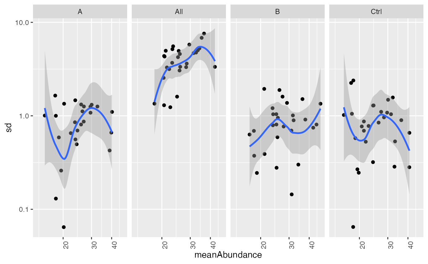

Scatter plot of standard deviation vs mean

Normalize protein intensities

Next, we want to normalize the data by first \(\log_2\) transforming it and then z-scaling. The \(log_2\) stabilizes the variance, while the z-scaling removes systematic differences from the samples.

lt <- lfqdata$get_Transformer()
transformed <- lt$log2()$robscale()$lfq
transformed$config$table$is_response_transformed

## [1] TRUE

Again we want to look into the distribution of the intensities in our samples after normalization.

pl <- transformed$get_Plotter()
pl$intensity_distribution_density()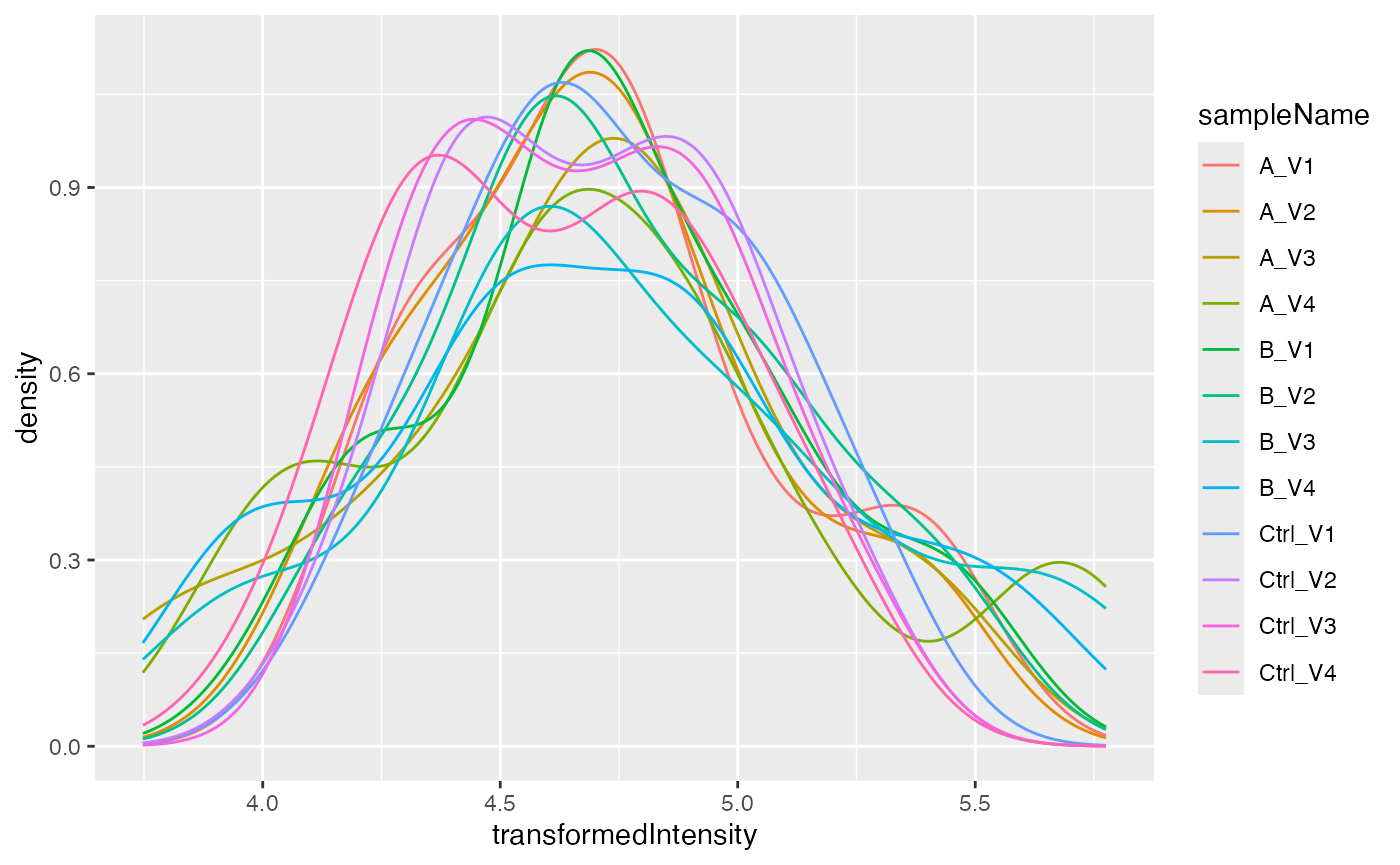

Normalized intensities.

plots matrix scatter plot in the upper right matrix and some statistics in the lower left matrix.

pl$pairs_smooth()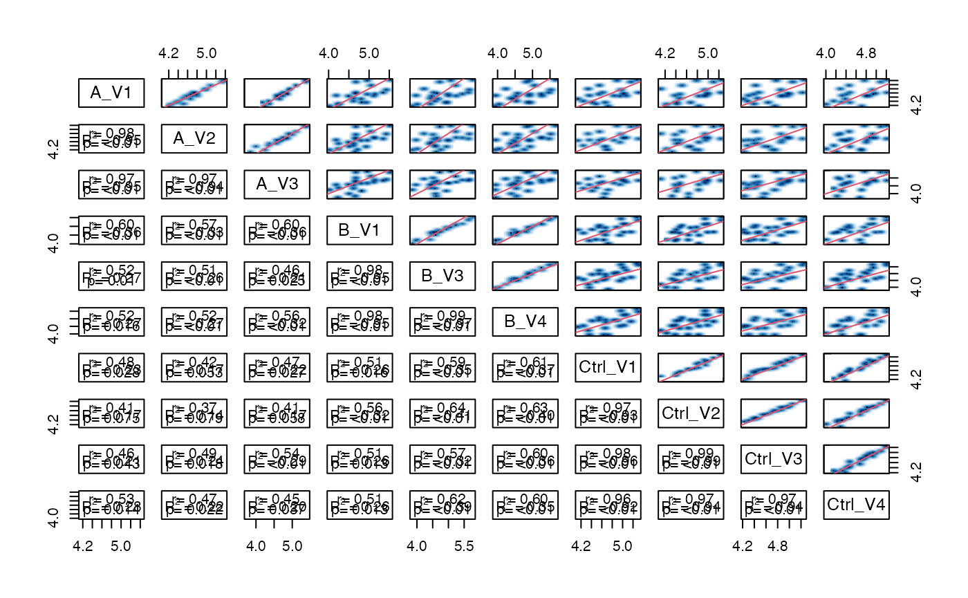

Scatterplot matrix

## NULL

plots protein heatmap:

p <- pl$heatmap() 
p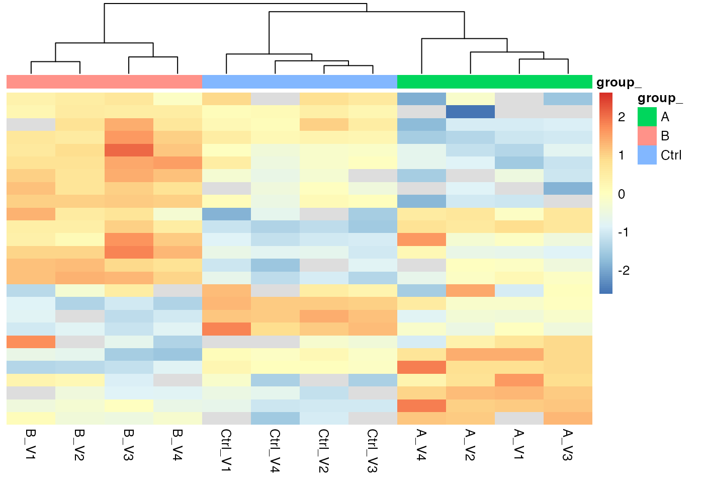

Heatmap, Rows - proteins, Columns - samples

We can also look at the correlation among the samples or look at a PCA plot.

hc <- pl$heatmap_cor()

hc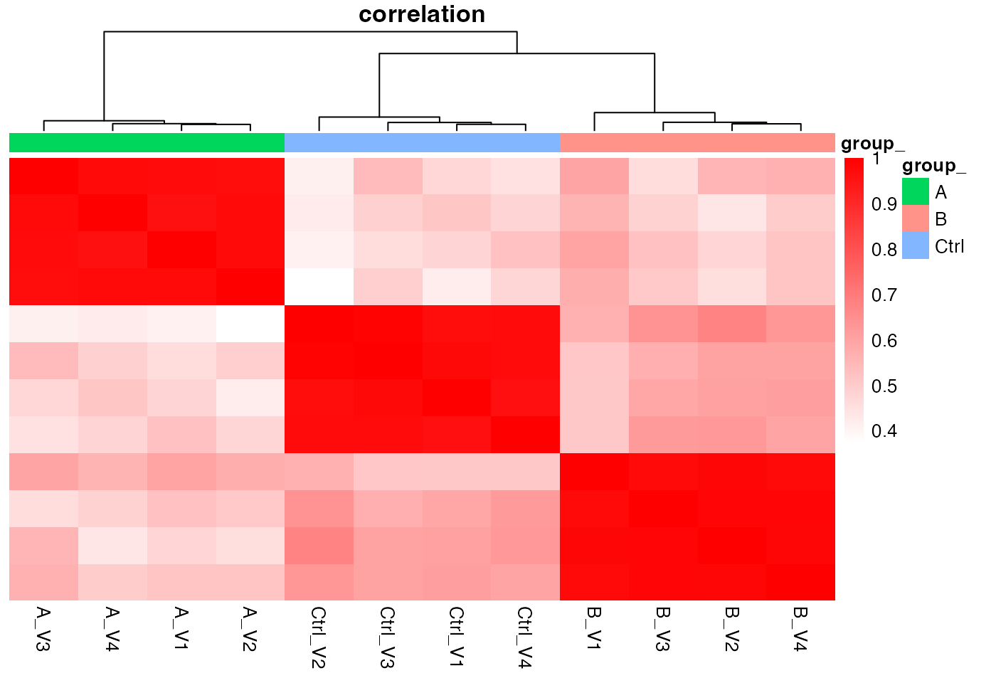

Heatmap based on sample correlations, Rows - samples, Columns - samples

pl$pca()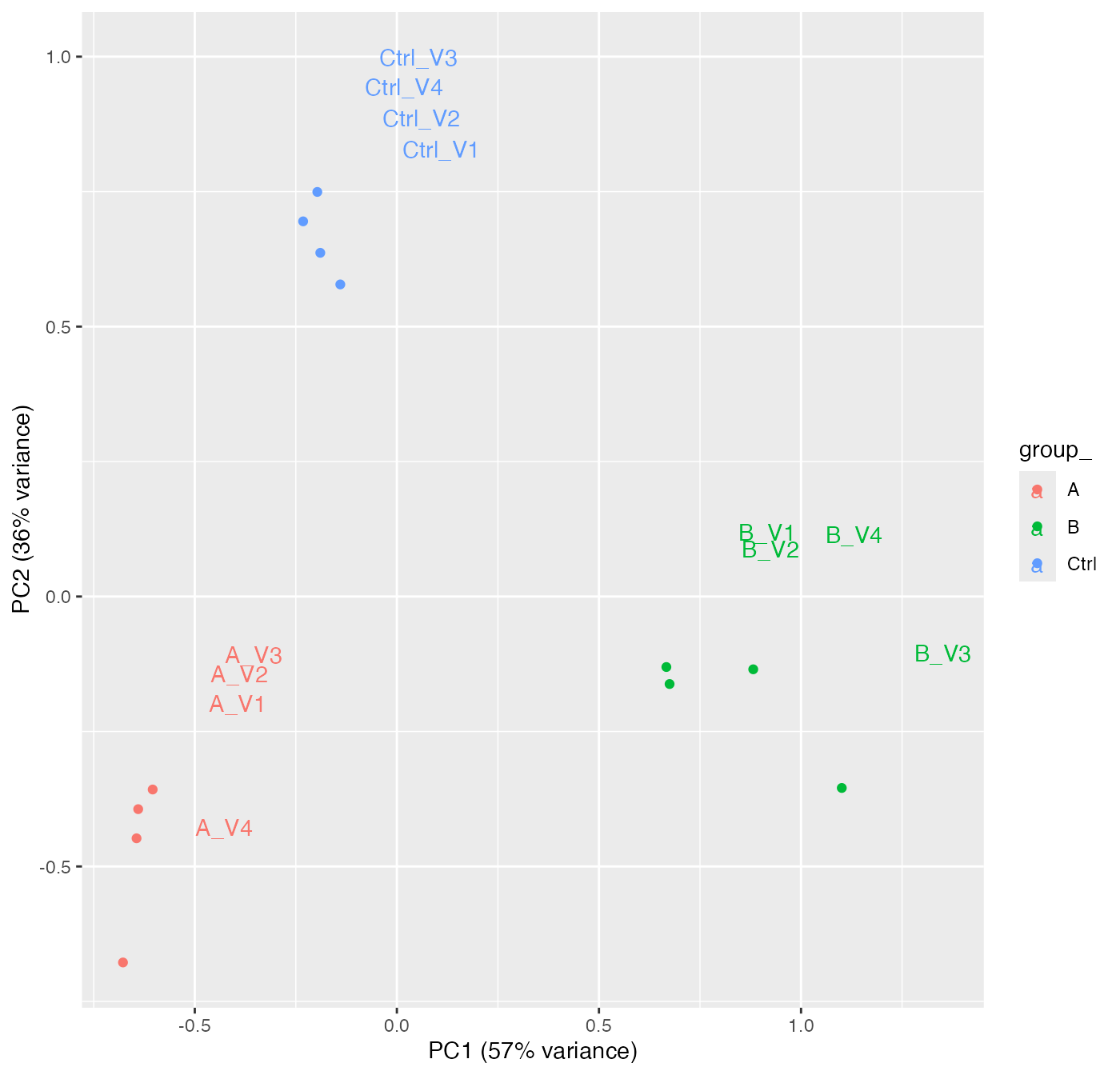

Principal component analysis for all samples

prints the standard deviations:

stats <- transformed$get_Stats()

## [1] "group_"
## NULL

prolfqua::table_facade(stats$stats_quantiles()$wide, "Standard deviations")

Standard deviations
probs	A	All	B	Ctrl
0.10	0.0355196	0.1152932	0.0325012	0.0294799
0.25	0.0587524	0.1677154	0.0582281	0.0422670
0.50	0.0717438	0.2345489	0.0853025	0.0566645
0.75	0.1240478	0.3004859	0.1209993	0.0720238
0.90	0.1687990	0.3253740	0.1388753	0.1087199

plots density of the standard deviation

stats$density_median()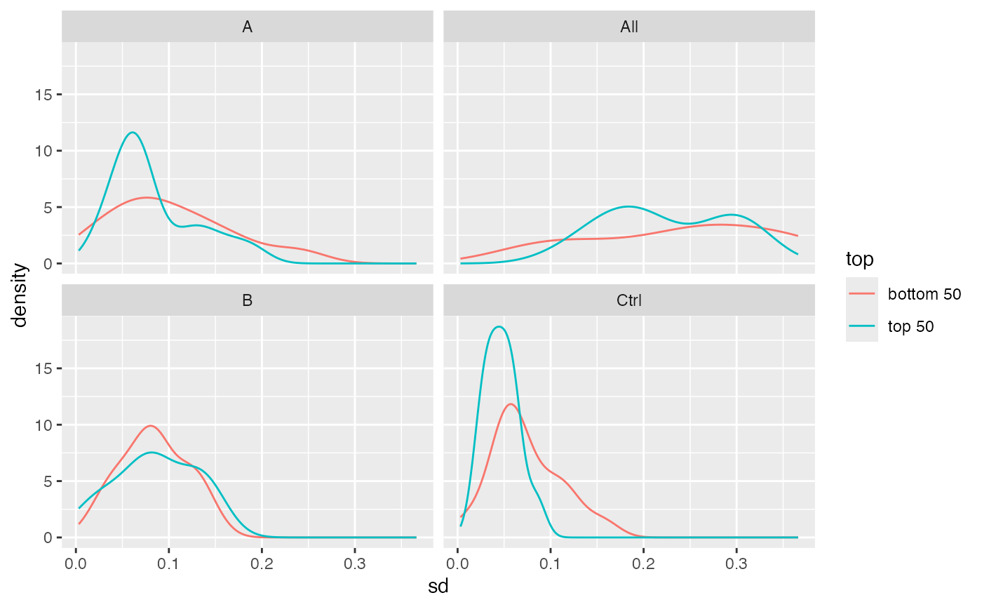

Density of the standard deviation

Check for heteroskedasticity. After transformation, the standard deviation should be independent of the mean intensity.

stdm_trans <- stats$stdv_vs_mean(size = 10000) + ggplot2::scale_x_log10() + ggplot2::scale_y_log10()
stdm_trans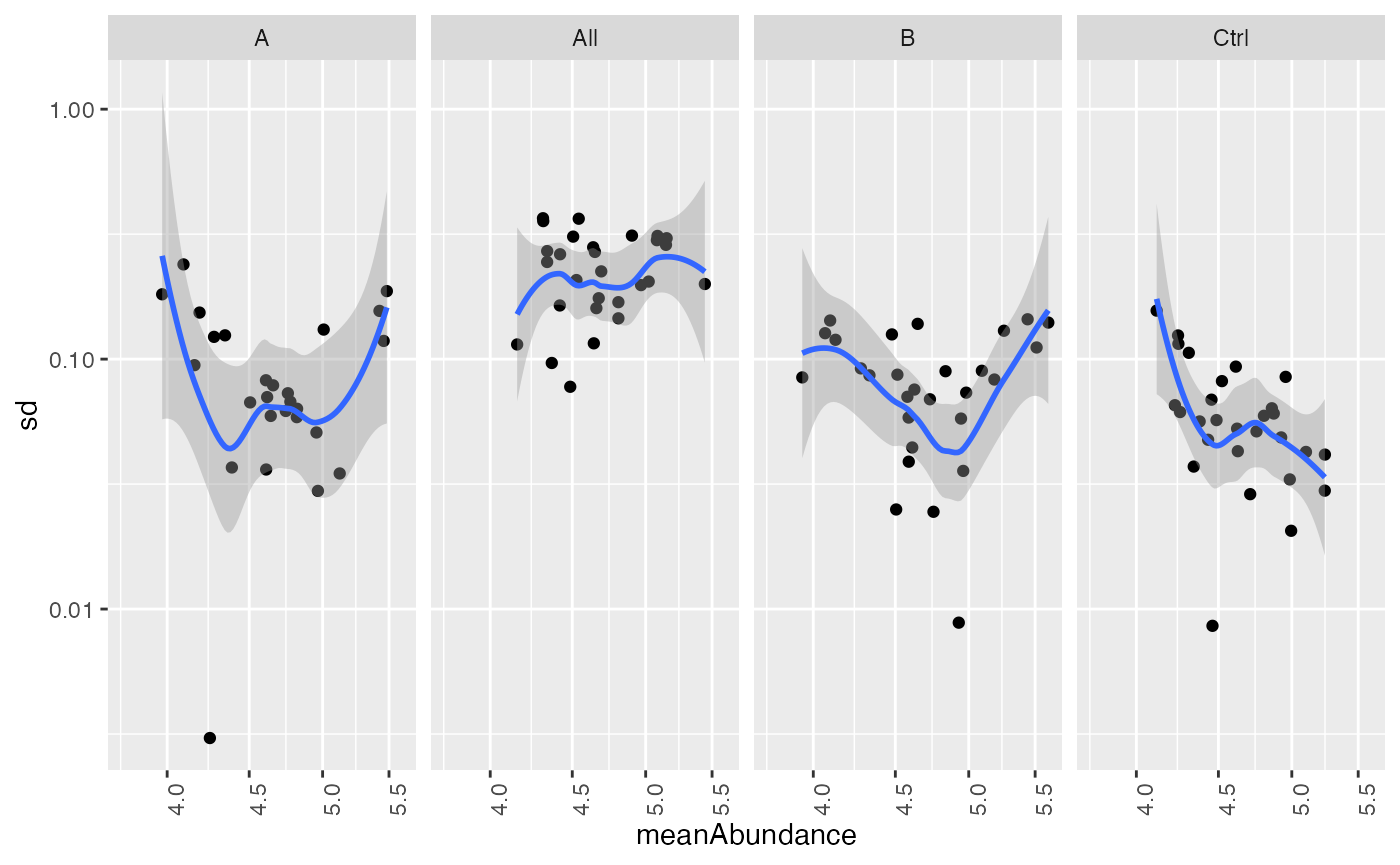

Scatter plot of sd vs mean of protein intensity

#gridExtra::grid.arrange(stdm_raw, stdm_trans, nrow=1)

Estimate sample size

For the sample size estimation we will now focus on only one condition and the different bio-reps from the a group In this condition all samples have the same concentration and we want to check variability within this group. Like this we can estimate how many samples are necessary per group to quantify properly a two-fold change (delta of 1) for 90% of all the proteins with a power of 0.8 and significance level of 0.05.

First, we need to filter our data for group_ A only.

transformedA <- transformed$get_copy()
transformedA$data <- transformedA$data |> dplyr::filter(group_  == "A")
stats <- transformedA$get_Stats()

## [1] "group_"
## NULL

stats$density(ggstat = "ecdf")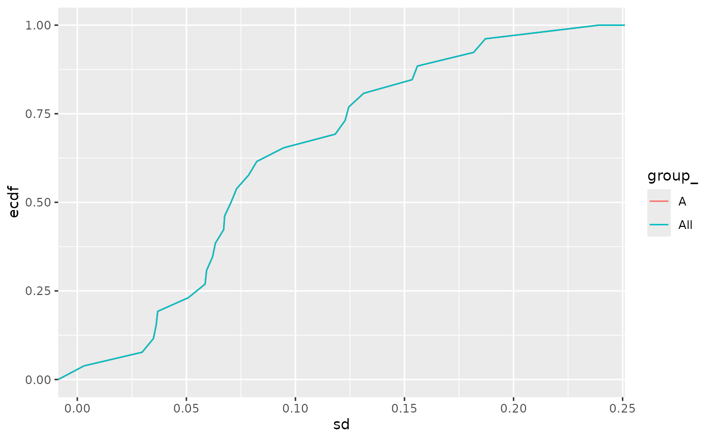

Empirical cumulative density function of the standard deviation for all the proteins in the dataset.

The table indicates that for this kind of data - if a two-fold change for 90% of all the proteins should be accurately quantified with a power of 0.8 (at 0.05 significance level) one would need to have 10 samples in each group.

sampleSize <- stats$power_t_test_quantiles() |> 
  dplyr::filter(group_ != "All")
prolfqua::table_facade(sampleSize, "Sample sizes. delta - Effect size, N - samplesize")

Sample sizes. delta - Effect size, N - samplesize
group_	probs	quantiles	sdtrimmed	N_exact	N	delta
A	0.10	0.0355196	0.0355196	1.526948	2	0.59
A	0.25	0.0587524	0.0587524	1.673109	2	0.59
A	0.50	0.0717438	0.0717438	1.758418	2	0.59
A	0.75	0.1240478	0.1240478	2.172950	3	0.59
A	0.90	0.1687990	0.1687990	2.671229	3	0.59
A	0.10	0.0355196	0.0530265	1.500024	2	1.00
A	0.25	0.0587524	0.0587524	1.521541	2	1.00
A	0.50	0.0717438	0.0717438	1.569649	2	1.00
A	0.75	0.1240478	0.1240478	1.768204	2	1.00
A	0.90	0.1687990	0.1687990	1.961551	2	1.00
A	0.10	0.0355196	0.1060530	1.500024	2	2.00
A	0.25	0.0587524	0.1060530	1.500024	2	2.00
A	0.50	0.0717438	0.1060530	1.500024	2	2.00
A	0.75	0.1240478	0.1240478	1.533718	2	2.00
A	0.90	0.1687990	0.1687990	1.616344	2	2.00

The table summarises visually how many samples are needed for different expected differences (in log2-scale) and different portions of all proteins.

sampleSize |>
  ggplot2::ggplot(ggplot2::aes(x = factor(probs) , y = N)) +
  ggplot2::facet_wrap(~delta) +
  ggplot2::geom_bar(stat = "identity")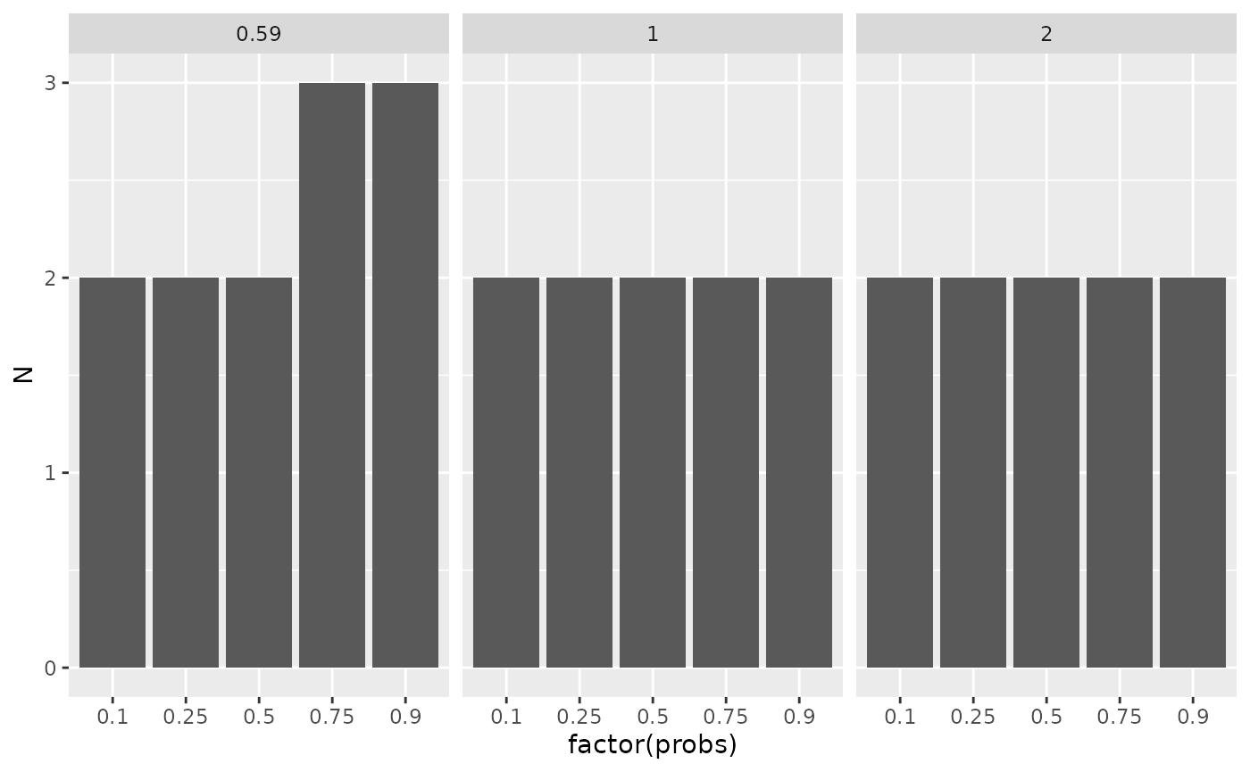

Estimated sample sizes for various FC levels and various quantiles of the standard deviation.

It is also possible to get the statistics for each protein in each group. The information includes group size, number of observations, standard deviation, variance, mean.

stats$stats() |> head()

## # A tibble: 6 × 11
##   protein_Id  peptide_Id group_ nrReplicates nrMeasured nrNAs      sd        var
##   <chr>       <chr>      <chr>         <int>      <int> <int>   <dbl>      <dbl>
## 1 0EfVhX~0087 ITLb4x1q   A                 4          3     1 0.154   0.0236    
## 2 0EfVhX~0087 ahQLlQY7   A                 4          4     0 0.0620  0.00385   
## 3 0EfVhX~0087 dJkdz7so   A                 4          2     2 0.182   0.0330    
## 4 7cbcrd~5725 D5dQ4nKk   A                 4          4     0 0.0509  0.00259   
## 5 9VUkAq~4703 eIC06D7g   A                 4          4     0 0.0946  0.00895   
## 6 BEJI92~5282 HBkZvdhT   A                 4          2     2 0.00305 0.00000929
## # ℹ 3 more variables: meanAbundance <dbl>, medianAbundance <dbl>,
## #   interaction <chr>

You can also estimate the sample size needed to perform differential expression analysis for each protein, given the power, delta, and sig.level. The next figure shows the distribution of needed sample sizes for all proteins with a power of 0.8 at signifiance level 0.05 for a two fold change (delta = 1).

x <- stats$power_t_test(delta = 1,power = 0.8, sig.level = 0.05)
x <- x |> dplyr::filter(group_ == "A") |> dplyr::arrange(desc(N),protein_Id)
prolfqua::table_facade(x[1:7,], caption = "Sample size for each protein")

Sample size for each protein
protein_Id	peptide_Id	group_	nrReplicates	nrMeasured	nrNAs	sd	var	meanAbundance	medianAbundance	interaction	delta	N_exact	N
0EfVhX~0087	dJkdz7so	A	4	2	2	0.1816806	0.0330078	3.971469	3.971469	group_A	1	2.023422	3
HvIpHG~9079	opjydeWJ	A	4	3	1	0.2392614	0.0572460	4.094835	3.997946	group_A	1	2.344670	3
JcKVfU~9653	9LMQBevj	A	4	4	0	0.1871014	0.0350069	5.482917	5.406550	group_A	1	2.050429	3
0EfVhX~0087	ITLb4x1q	A	4	3	1	0.1535287	0.0235710	4.190351	4.178250	group_A	1	1.892113	2
0EfVhX~0087	ahQLlQY7	A	4	4	0	0.0620097	0.0038452	4.742744	4.735435	group_A	1	1.533666	2
7cbcrd~5725	D5dQ4nKk	A	4	4	0	0.0508679	0.0025875	4.956022	4.964554	group_A	1	1.500024	2
9VUkAq~4703	eIC06D7g	A	4	4	0	0.0945821	0.0089458	4.159728	4.182873	group_A	1	1.654299	2

x |> ggplot2::ggplot(ggplot2::aes(x = N)) +
  ggplot2::geom_histogram() +
  ggplot2::facet_wrap(~delta) +
  ggplot2::xlim(0,100)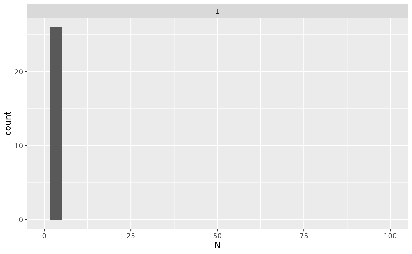

Distribution of the required sample sizes for two fold change thresholds for all the proteins.

The prolfqua package is described in (Wolski et al. 2022).

Session Info

sessionInfo()

## R version 4.3.2 (2023-10-31)
## Platform: aarch64-apple-darwin20 (64-bit)
## Running under: macOS Sonoma 14.5
## 
## Matrix products: default
## BLAS:   /Library/Frameworks/R.framework/Versions/4.3-arm64/Resources/lib/libRblas.0.dylib 
## LAPACK: /Library/Frameworks/R.framework/Versions/4.3-arm64/Resources/lib/libRlapack.dylib;  LAPACK version 3.11.0
## 
## locale:
## [1] en_US.UTF-8/en_US.UTF-8/en_US.UTF-8/C/en_US.UTF-8/en_US.UTF-8
## 
## time zone: Europe/Zurich
## tzcode source: internal
## 
## attached base packages:
## [1] stats     graphics  grDevices utils     datasets  methods   base     
## 
## loaded via a namespace (and not attached):
##  [1] tidyr_1.3.1        plotly_4.10.4      sass_0.4.9         utf8_1.2.4        
##  [5] generics_0.1.3     KernSmooth_2.23-22 lattice_0.22-5     stringi_1.8.3     
##  [9] digest_0.6.35      magrittr_2.0.3     evaluate_0.23      grid_4.3.2        
## [13] RColorBrewer_1.1-3 fastmap_1.1.1      Matrix_1.6-5       jsonlite_1.8.8    
## [17] ggrepel_0.9.5      prolfqua_1.2.5     conflicted_1.2.0   gridExtra_2.3     
## [21] mgcv_1.9-1         httr_1.4.7         purrr_1.0.2        fansi_1.0.6       
## [25] viridisLite_0.4.2  scales_1.3.0       lazyeval_0.2.2     textshaping_0.3.7 
## [29] jquerylib_0.1.4    cli_3.6.2          rlang_1.1.3        splines_4.3.2     
## [33] munsell_0.5.1      withr_3.0.0        cachem_1.0.8       yaml_2.3.8        
## [37] tools_4.3.2        memoise_2.0.1      dplyr_1.1.4        colorspace_2.1-0  
## [41] ggplot2_3.5.1      forcats_1.0.0      vctrs_0.6.5        R6_2.5.1          
## [45] lifecycle_1.0.4    stringr_1.5.1      fs_1.6.4           htmlwidgets_1.6.4 
## [49] MASS_7.3-60.0.1    ragg_1.3.0         pkgconfig_2.0.3    desc_1.4.3        
## [53] pkgdown_2.0.9      pillar_1.9.0       bslib_0.7.0        gtable_0.3.5      
## [57] glue_1.7.0         data.table_1.15.4  Rcpp_1.0.12        systemfonts_1.0.6 
## [61] highr_0.10         xfun_0.43          tibble_3.2.1       tidyselect_1.2.1  
## [65] knitr_1.46         farver_2.1.1       nlme_3.1-164       htmltools_0.5.8.1 
## [69] labeling_0.4.3     rmarkdown_2.26     pheatmap_1.0.12    compiler_4.3.2

References

Wolski, Witold E., Paolo Nanni, Jonas Grossmann, Maria d’Errico, Ralph Schlapbach, and Christian Panse. 2022. “Prolfqua: A Comprehensive R-package for Proteomics Differential Expression Analysis.” bioRxiv. https://doi.org/10.1101/2022.06.07.494524.

Witold E. Wolski

2024-05-30