Simulate Peptide level Data

Dimulate data

For proteins: - the proteins have a FC either equal 1, 0. or -1, 10% have 1 80% have 0 and 10% have -1.

What we however are measuring are peptide spectrum matches. Let’s assume we observing peptides.

For peptides:

The transformed protein abundances have a log normal distribution with meanlog = log(20), and sd = log(1.2).
The number of peptides per protein follow a geometric distribution, $N_{pep} \sim Geo(p)$ with $p = 0.3$
The peptide abundances of a protein have log normal distribution with meanlog = log(proteinabundance) and sd = log(1.2)
The log2 intensities of a peptide within a group follow a normal distribution distribution $I_{pep} LogNormal(,) $, where $\mu$ is the peptide abundance and $\sigma$

peptideAbundances <- prolfqua::sim_lfq_data(PEPTIDE = TRUE)

Analyse simulated data with prolfqua

library(prolfqua)

config <- AnalysisConfiguration$new()
config$file_name = "sample"
config$factors["group_"] = "group"
config$hierarchy[["protein_Id"]] = "proteinID"
config$hierarchy[["peptide_Id"]] = "peptideID"
config$set_response("abundance")

adata <- setup_analysis(peptideAbundances, config)

lfqdata <- prolfqua::LFQData$new(adata, config)
lfqdata$is_transformed(TRUE)

lfqdata$remove_small_intensities(threshold = 1)
lfqdata$filter_proteins_by_peptide_count()

lfqdata$factors()

## # A tibble: 12 × 3
##    sample  sampleName group_
##    <chr>   <chr>      <chr> 
##  1 A_V1    A_V1       A     
##  2 A_V2    A_V2       A     
##  3 A_V3    A_V3       A     
##  4 A_V4    A_V4       A     
##  5 B_V1    B_V1       B     
##  6 B_V2    B_V2       B     
##  7 B_V3    B_V3       B     
##  8 B_V4    B_V4       B     
##  9 Ctrl_V1 Ctrl_V1    Ctrl  
## 10 Ctrl_V2 Ctrl_V2    Ctrl  
## 11 Ctrl_V3 Ctrl_V3    Ctrl  
## 12 Ctrl_V4 Ctrl_V4    Ctrl

pl <- lfqdata$get_Plotter()
lfqdata$hierarchy_counts()

## # A tibble: 1 × 3
##   isotopeLabel protein_Id peptide_Id
##   <chr>             <int>      <int>
## 1 light                16         60

lfqdata$relevant_hierarchy_keys()

## [1] "protein_Id"

pl$heatmap()

pl$intensity_distribution_density()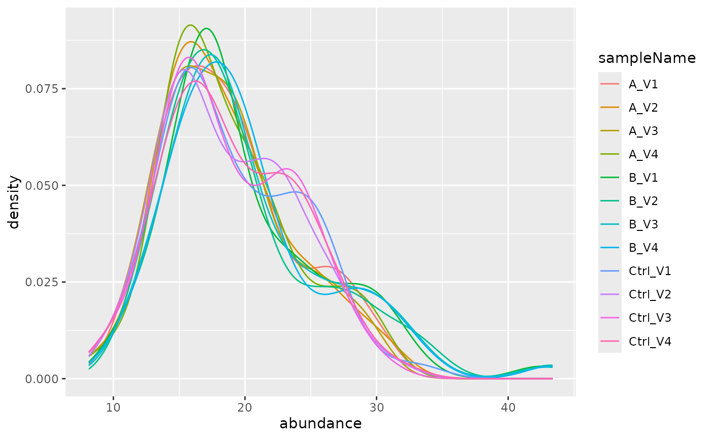

Fit peptide model

formula_Condition <-  strategy_lm("abundance ~ group_")
lfqdata$set_config_value("hierarchy_depth", 2)

# specify model definition
modelName  <- "Model"
contr_spec <- c("B_over_Ctrl" = "group_B - group_Ctrl",
               "A_over_Ctrl" = "group_A - group_Ctrl")
lfqdata$subject_id()

## [1] "protein_Id" "peptide_Id"

mod <- prolfqua::build_model(
  lfqdata,
  formula_Condition)
aovtable <- mod$get_anova()
mod$anova_histogram()$plot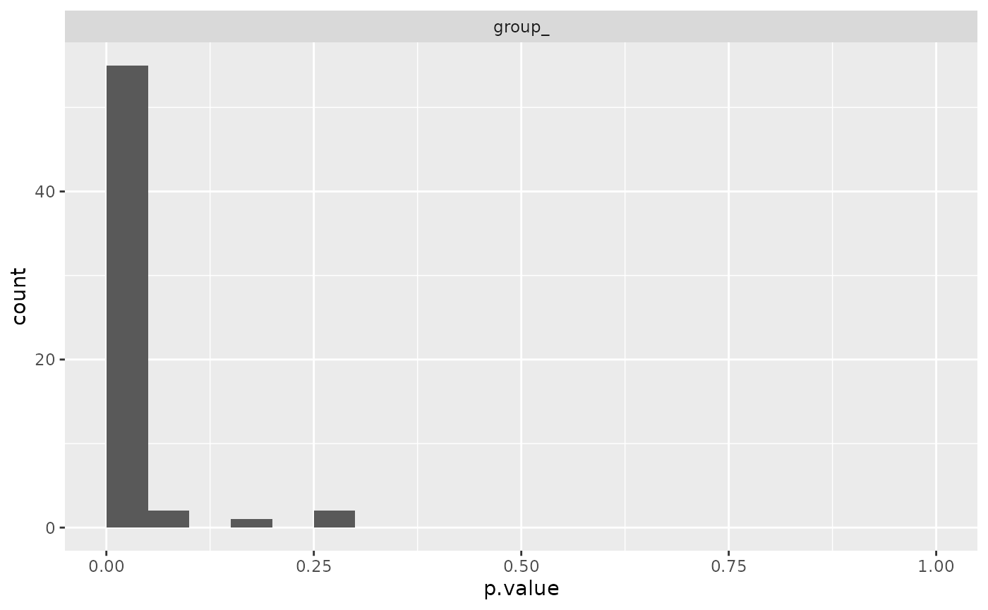

xx <- aovtable |> dplyr::filter(FDR < 0.05)
signif <- lfqdata$get_copy()
signif$set_data(signif$data_long() |> dplyr::filter(protein_Id %in% xx$protein_Id))
signif$get_Plotter()$heatmap()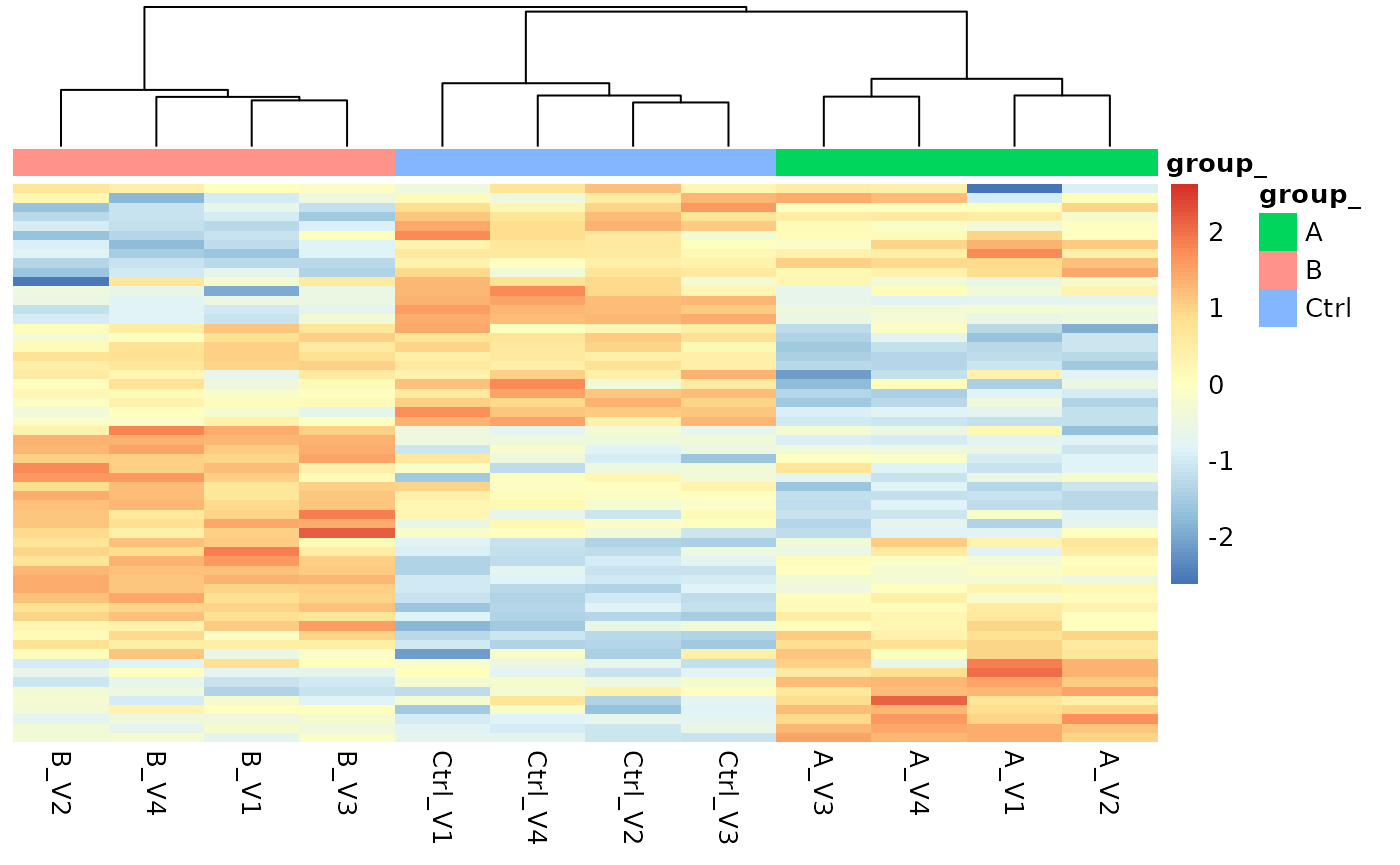

Aggregate data

lfqdata$set_config_value("hierarchy_depth", 1)
protData <- lfqdata$get_Aggregator()$aggregate()

protData$response()

## [1] "medpolish"

formula_Condition <-  strategy_lm("medpolish ~ group_")

mod <- prolfqua::build_model(
  protData,
  formula_Condition)

contr <- prolfqua::Contrasts$new(mod, contr_spec)
v1 <- contr$get_Plotter()$volcano()
v1$FDR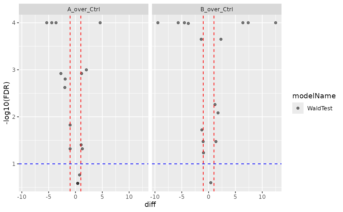

ctr <- contr$get_contrasts()

Session Info

sessionInfo()

## R version 4.5.2 (2025-10-31)
## Platform: x86_64-pc-linux-gnu
## Running under: Ubuntu 24.04.4 LTS
## 
## Matrix products: default
## BLAS:   /usr/lib/x86_64-linux-gnu/openblas-pthread/libblas.so.3 
## LAPACK: /usr/lib/x86_64-linux-gnu/openblas-pthread/libopenblasp-r0.3.26.so;  LAPACK version 3.12.0
## 
## locale:
##  [1] LC_CTYPE=C.UTF-8       LC_NUMERIC=C           LC_TIME=C.UTF-8       
##  [4] LC_COLLATE=C.UTF-8     LC_MONETARY=C.UTF-8    LC_MESSAGES=C.UTF-8   
##  [7] LC_PAPER=C.UTF-8       LC_NAME=C              LC_ADDRESS=C          
## [10] LC_TELEPHONE=C         LC_MEASUREMENT=C.UTF-8 LC_IDENTIFICATION=C   
## 
## time zone: UTC
## tzcode source: system (glibc)
## 
## attached base packages:
## [1] stats     graphics  grDevices utils     datasets  methods   base     
## 
## other attached packages:
## [1] prolfqua_1.6.1
## 
## loaded via a namespace (and not attached):
##  [1] tidyselect_1.2.1       viridisLite_0.4.3      dplyr_1.2.1           
##  [4] farver_2.1.2           S7_0.2.2               fastmap_1.2.0         
##  [7] lazyeval_0.2.3         digest_0.6.39          rpart_4.1.24          
## [10] lifecycle_1.0.5        survival_3.8-3         statmod_1.5.1         
## [13] magrittr_2.0.5         compiler_4.5.2         progress_1.2.3        
## [16] rlang_1.2.0            sass_0.4.10            tools_4.5.2           
## [19] utf8_1.2.6             yaml_2.3.12            data.table_1.18.2.1   
## [22] knitr_1.51             prettyunits_1.2.0      labeling_0.4.3        
## [25] htmlwidgets_1.6.4      plyr_1.8.9             RColorBrewer_1.1-3    
## [28] withr_3.0.2            purrr_1.2.2            desc_1.4.3            
## [31] nnet_7.3-20            grid_4.5.2             jomo_2.7-6            
## [34] mice_3.19.0            ggplot2_4.0.3          scales_1.4.0          
## [37] iterators_1.0.14       MASS_7.3-65            cli_3.6.6             
## [40] crayon_1.5.3           UpSetR_1.4.0           rmarkdown_2.31        
## [43] ragg_1.5.2             reformulas_0.4.4       generics_0.1.4        
## [46] otel_0.2.0             httr_1.4.8             minqa_1.2.8           
## [49] cachem_1.1.0           operator.tools_1.6.3.1 splines_4.5.2         
## [52] vctrs_0.7.3            boot_1.3-32            glmnet_5.0            
## [55] Matrix_1.7-4           jsonlite_2.0.0         hms_1.1.4             
## [58] mitml_0.4-5            ggrepel_0.9.8          systemfonts_1.3.2     
## [61] foreach_1.5.2          limma_3.66.0           plotly_4.12.0         
## [64] tidyr_1.3.2            jquerylib_0.1.4        glue_1.8.1            
## [67] pkgdown_2.2.0          nloptr_2.2.1           pan_1.9               
## [70] codetools_0.2-20       stringi_1.8.7          shape_1.4.6.1         
## [73] gtable_0.3.6           lme4_2.0-1             tibble_3.3.1          
## [76] pillar_1.11.1          htmltools_0.5.9        R6_2.6.1              
## [79] textshaping_1.0.5      Rdpack_2.6.6           formula.tools_1.7.1   
## [82] evaluate_1.0.5         lattice_0.22-7         rbibutils_2.4.1       
## [85] backports_1.5.1        pheatmap_1.0.13        broom_1.0.12          
## [88] bslib_0.10.0           Rcpp_1.1.1-1.1         gridExtra_2.3         
## [91] nlme_3.1-168           mgcv_1.9-3             logistf_1.26.1        
## [94] xfun_0.57              fs_2.1.0               forcats_1.0.1         
## [97] pkgconfig_2.0.3

Witold E. Wolski

2026-05-06

Dimulate data

Analyse simulated data with prolfqua

Fit peptide model

Aggregate data

Session Info