Introduction to prolfqua
Witold E. Wolski
Functional Genomics Center Zurich (FGCZ), ETH Zurich and University of ZurichSource:
vignettes/prolfqua.Rmd
prolfqua.Rmd
Documentation
The vignettes of this package, in reading order:
- Introduction to prolfqua (this vignette)
-
Importing your data:
reading your own data into an
AnalysisConfiguration -
Comparing two groups: QC,
normalization and contrasts with
lm_impute -
All modelling methods at a
glance: every
build_contrast_analysis()method on one small dataset - Two-factor designs
- Contrasts from factors
-
Filling the gaps: model-based
imputation for heatmaps and PCA: completing the data matrix with
impute_from_model() - QC and sample size estimation
The package website https://fgcz.github.io/prolfqua/ has three more articles:
-
Comparing
modelling methods on one dataset: all
build_contrast_analysis()methods side by side, with plots - Simulating peptide-level data
-
Under
the hood: strategy, model and contrasts: the classes behind
build_contrast_analysis()
Introduction
prolfqua covers the steps of a label-free quantification (LFQ) proteomics analysis: quality control, normalization, aggregation of peptides to proteins, modelling, hypothesis testing and sample size estimation (Wolski et al. 2023).
The centre of the package is a factory,
build_contrast_analysis(). It takes the data, a model
formula, the contrasts and a method, and returns a ready
analysis: one model per protein and the requested contrasts.
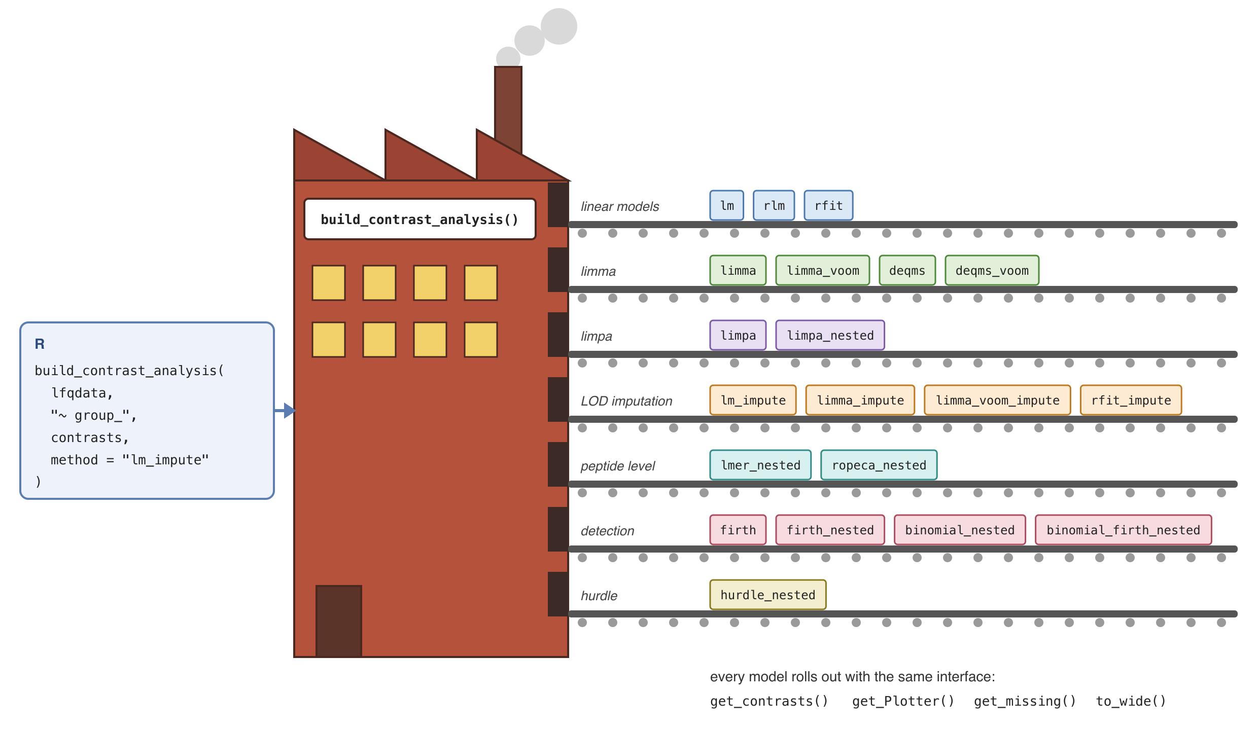
build_contrast_analysis() is a factory: the method key selects the model, and every model rolls out with the same interface.
The method argument selects the model: linear models
(lm, rlm, rfit), limma and
limma-voom, DEqMS variance moderation, limpa’s detection probability
model, Firth logistic and binomial models of detection, mixed models and
ROPECA on peptide-level data, a hurdle model combining intensity and
detection, and variants that impute groups without observations at the
limit of detection.
Every method returns an object with the same interface:
get_contrasts(), get_Plotter(),
get_missing() and to_wide(). Results of
different methods therefore have the same columns and can be compared or
combined directly.
build_contrast_analysis() takes its data as an
LFQData object. The package works with data in long format,
one row per measured feature (protein, peptide, precursor) and
sample:
-
AnalysisConfigurationmaps the columns of the table to their roles: the feature hierarchy (protein, peptide, …), the explanatory factors, the sample and the intensity column. -
LFQDataholds the data together with its configuration. Its methods return helpers for transformation (get_Transformer()), aggregation (get_Aggregator()), summary statistics (get_Stats()), missing-value summaries (get_Summariser()) and plots (get_Plotter()).
Installation
Install prolfqua from Bioconductor with:
if (!requireNamespace("BiocManager", quietly = TRUE)) {
  install.packages("BiocManager")
}
BiocManager::install("prolfqua")
The development version is available on GitHub:
BiocManager::install("fgcz/prolfqua")Quick start
We simulate peptide-level intensities for 100 proteins measured in
three groups (A, B and Ctrl).
sim_lfq_data_peptide_config() returns the data together
with a matching AnalysisConfiguration.
library(prolfqua)
istar <- sim_lfq_data_peptide_config(Nprot = 100, seed = 1234)
lfqdata <- LFQData$new(istar$data, istar$config)
lfqdata$factors() |> head()
#> # A tibble: 6 × 3
#>   sample sampleName group_
#>   <chr>  <chr>      <chr>
#> 1 A_V1   A_V1       A
#> 2 A_V2   A_V2       A
#> 3 A_V3   A_V3       A
#> 4 A_V4   A_V4       A
#> 5 B_V1   B_V1       B
#> 6 B_V2   B_V2       B
We transform the intensities, scale them robustly, and aggregate the peptides to proteins with Tukey’s median polish.
lfqdata <- lfqdata$get_Transformer()$log2()$robscale()$lfq
lfqprot <- lfqdata$get_Aggregator()$aggregate()
lfqprot$get_Plotter()$intensity_distribution_density()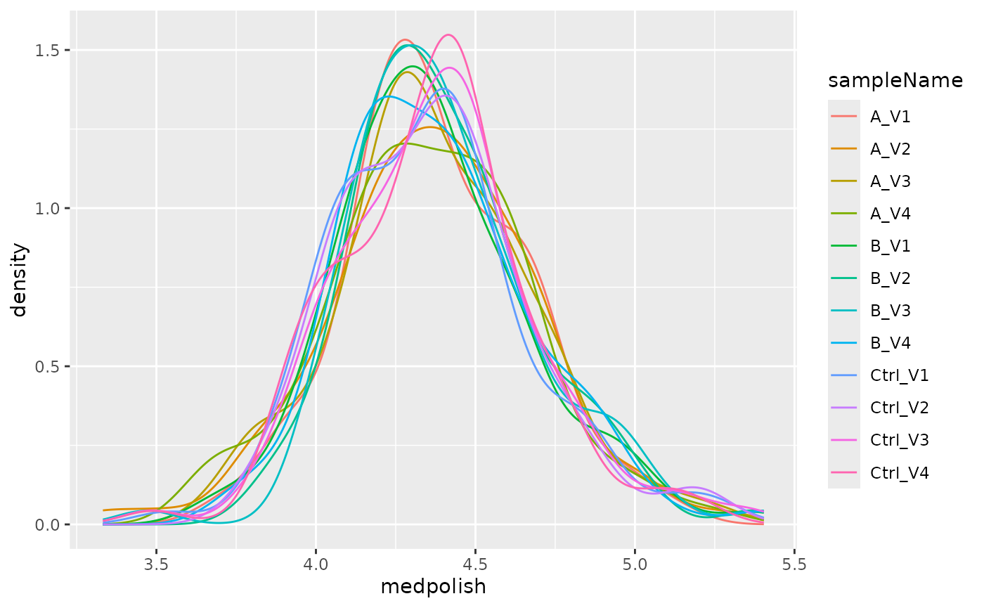
Distribution of the normalized protein intensities per sample.
We compare groups A and B with the control
group using lm_impute: a linear model per protein with
moderated variances. Proteins whose fit fails because a group has no
observations are refitted with the missing values imputed at the limit
of detection, borrowing the variance from the other proteins.
contrasts <- c(
  "A_vs_Ctrl" = "group_A - group_Ctrl",
  "B_vs_Ctrl" = "group_B - group_Ctrl"
)
fa <- build_contrast_analysis(lfqprot, "~ group_", contrasts, method = "lm_impute")
res <- fa$get_contrasts()
head(res[, c("protein_Id", "contrast", "diff", "p.value", "FDR")])
#> # A tibble: 6 × 5
#>   protein_Id  contrast     diff    p.value       FDR
#>   <chr>       <chr>       <dbl>      <dbl>     <dbl>
#> 1 0EfVhX~3967 A_vs_Ctrl  0.199  0.000123   0.000397
#> 2 0m5WN4~6025 A_vs_Ctrl  0.178  0.0000160  0.0000726
#> 3 0YSKpy~2865 A_vs_Ctrl -0.175  0.00277    0.00554
#> 4 3QLHfm~8938 A_vs_Ctrl  0.214  0.00456    0.00807
#> 5 3QYop0~7543 A_vs_Ctrl -0.221  0.00000298 0.0000179
#> 6 76k03k~7094 A_vs_Ctrl -0.0822 0.00980    0.0156
fa$get_Plotter()$volcano()$FDR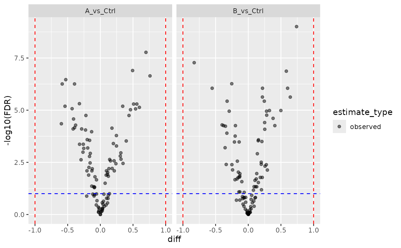
Volcano plot of the two contrasts.
All available methods are listed by list_facades(); the
vignette All modelling methods at a
glance runs each of them on one small dataset.
names(list_facades())
#>  [1] "binomial_firth_nested" "binomial_nested"       "deqms"
#>  [4] "deqms_voom"            "firth"                 "firth_nested"
#>  [7] "hurdle_nested"         "limma"                 "limma_impute"
#> [10] "limma_voom"            "limma_voom_impute"     "limpa"
#> [13] "limpa_nested"          "lm"                    "lm_impute"
#> [16] "lmer_nested"           "rfit"                  "rfit_impute"
#> [19] "rlm"                   "ropeca_nested"
Session info
sessionInfo()
#> R version 4.6.2 (2026-10-29)
#> Platform: x86_64-pc-linux-gnu
#> Running under: Ubuntu 26.04.1 LTS
#>
#> Matrix products: default
#> BLAS:   /usr/lib/x86_64-linux-gnu/openblas-pthread/libblas.so.3
#> LAPACK: /usr/lib/x86_64-linux-gnu/openblas-pthread/libopenblasp-r0.3.32.so;  LAPACK version 3.12.0
#>
#> locale:
#>  [1] LC_CTYPE=C.UTF-8       LC_NUMERIC=C           LC_TIME=C.UTF-8
#>  [4] LC_COLLATE=C.UTF-8     LC_MONETARY=C.UTF-8    LC_MESSAGES=C.UTF-8
#>  [7] LC_PAPER=C.UTF-8       LC_NAME=C              LC_ADDRESS=C
#> [10] LC_TELEPHONE=C         LC_MEASUREMENT=C.UTF-8 LC_IDENTIFICATION=C
#>
#> time zone: UTC
#> tzcode source: system (glibc)
#>
#> attached base packages:
#> [1] stats     graphics  grDevices utils     datasets  methods   base
#>
#> other attached packages:
#> [1] prolfqua_1.9.0   BiocStyle_2.40.0
#>
#> loaded via a namespace (and not attached):
#>   [1] Rdpack_2.6.6           gridExtra_2.3.1        rlang_1.3.0
#>   [4] magrittr_2.0.5         clue_0.3-68            GetoptLong_1.1.1
#>   [7] otel_0.2.0             matrixStats_1.5.0      compiler_4.6.2
#>  [10] mgcv_1.9-4             png_0.1-9              systemfonts_1.3.2
#>  [13] vctrs_0.7.3            pkgconfig_2.0.3        shape_1.4.6.1
#>  [16] crayon_1.5.3           fastmap_1.2.0          backports_1.5.1
#>  [19] labeling_0.4.3         utf8_1.2.6             promises_1.5.0
#>  [22] rmarkdown_2.32         nloptr_2.2.1           ragg_1.5.2
#>  [25] UpSetR_1.4.1           purrr_1.2.2            xfun_0.62
#>  [28] glmnet_5.2             jomo_2.7-6             logistf_1.26.1
#>  [31] cachem_1.1.0           jsonlite_2.0.0         progress_1.2.3
#>  [34] later_1.4.8            pan_2.0                prettyunits_1.2.0
#>  [37] broom_1.0.13           parallel_4.6.2         cluster_2.1.8.3
#>  [40] R6_2.6.1               stringi_1.8.9          bslib_0.12.0
#>  [43] RColorBrewer_1.1-3     limma_3.68.5           boot_1.3-32
#>  [46] rpart_4.1.27           jquerylib_0.1.4        Rcpp_1.1.2
#>  [49] bookdown_0.48          iterators_1.0.14       knitr_1.52
#>  [52] IRanges_2.46.0         httpuv_1.6.17          Matrix_1.7-6
#>  [55] splines_4.6.2          nnet_7.3-21            tidyselect_1.2.1
#>  [58] yaml_2.3.12            doParallel_1.0.17      codetools_0.2-20
#>  [61] lattice_0.23-1         tibble_3.3.1           plyr_1.8.9
#>  [64] shiny_1.14.0           withr_3.0.3            S7_0.2.2
#>  [67] evaluate_1.0.5         desc_1.4.3             survival_3.8-12
#>  [70] circlize_0.4.18        pillar_1.11.1          BiocManager_1.30.27
#>  [73] mice_3.19.0            foreach_1.5.2          stats4_4.6.2
#>  [76] reformulas_0.4.4       plotly_4.12.1          generics_0.1.4
#>  [79] hms_1.1.4              S4Vectors_0.50.3       ggplot2_4.0.3
#>  [82] scales_1.4.0           minqa_1.2.8            xtable_1.8-8
#>  [85] glue_1.8.1             tools_4.6.2            data.table_1.18.6.1
#>  [88] lme4_2.1-0             forcats_1.0.1          fs_2.1.0
#>  [91] grid_4.6.2             tidyr_1.3.2            crosstalk_1.2.2
#>  [94] rbibutils_2.4.1        colorspace_2.1-4       nlme_3.1-171
#>  [97] formula.tools_1.7.1    cli_3.6.6              textshaping_1.0.5
#> [100] viridisLite_0.4.3      ComplexHeatmap_2.28.0  dplyr_1.2.1
#> [103] gtable_0.3.6           sass_0.4.10            digest_0.6.39
#> [106] operator.tools_1.6.3.1 BiocGenerics_0.58.1    ggrepel_0.9.8
#> [109] rjson_0.2.23           htmlwidgets_1.6.4      farver_2.1.2
#> [112] htmltools_0.5.9        pkgdown_2.2.1          lifecycle_1.0.5
#> [115] httr_1.4.9             mime_0.13              GlobalOptions_0.1.4
#> [118] mitml_0.4-5            statmod_1.5.2          MASS_7.3-66