Absent, not unknown: proteins missing in a whole group
Witold E. Wolski
2026-10-29
Source:vignettes/articles/ModelBasedImputation.Rmd
ModelBasedImputation.RmdThe problem
In label-free data a protein is often not observed in any sample of
one group. Most of the time it is there, but below the limit of
detection (LOD): the absence is information, not an unknown value. A
linear model per protein cannot estimate a group without observations,
so lm drops exactly these contrasts, often the ones with
the largest changes.
library(prolfqua)
library(ggplot2)
sim <- sim_lfq_data_protein_config(Nprot = 100, weight_missing = 0.5, seed = 1234)
lfq <- LFQData$new(sim$data, sim$config)
contrasts <- c(AvsC = "group_A - group_Ctrl", BvsC = "group_B - group_Ctrl")

fa_lm <- build_contrast_analysis(lfq, "~ group_", contrasts, method = "lm")
lost <- fa_lm$get_missing()
lost
## # A tibble: 6 × 2
## protein_Id contrast
## <chr> <chr>
## 1 cnCfON~9769 BvsC
## 2 DoWup2~8058 BvsC
## 3 LMQBev~8107 AvsC
## 4 LMQBev~8107 BvsC
## 5 umjHSH~2090 AvsC
## 6 ZHBkZv~0394 AvsCThe intensities of these proteins show the empty groups:
lfq$data_long() |>
  dplyr::filter(protein_Id %in% lost$protein_Id) |>
  dplyr::select(protein_Id, sampleName, abundance) |>
  tidyr::pivot_wider(names_from = sampleName, values_from = abundance) |>
knitr::kable(digits = 1)| protein_Id | A_V1 | A_V2 | A_V3 | A_V4 | B_V1 | B_V2 | B_V3 | B_V4 | Ctrl_V1 | Ctrl_V2 | Ctrl_V3 | Ctrl_V4 |
|---|---|---|---|---|---|---|---|---|---|---|---|---|
| cnCfON~9769 | NA | 15.9 | 14.3 | 14.4 | NA | NA | NA | NA | NA | 15.8 | 17.5 | NA |
| DoWup2~8058 | 17.9 | NA | 18.9 | NA | NA | NA | NA | NA | NA | NA | NA | 17 |
| LMQBev~8107 | NA | 16.0 | NA | NA | NA | 15.8 | 16.0 | 15.8 | NA | NA | NA | NA |
| umjHSH~2090 | NA | NA | NA | NA | NA | NA | 15.8 | 16.5 | NA | NA | 17.4 | NA |
| ZHBkZv~0394 | NA | NA | NA | NA | NA | NA | NA | 13.3 | NA | NA | 12.6 | NA |
The limit of detection
MissingHelpers estimates the LOD from the data. Groups
in which a protein is observed in only one sample, or in the fewest
samples, are the closest the data comes to the detection limit; the LOD
is the median (prob = 0.5) of their mean intensities.
mh <- MissingHelpers$new(lfq$data_long(), lfq$get_config())
mh$get_lod()
## [1] 15.97769lm_impute
lm_impute fits lm to every protein.
Proteins whose fit fails, or leaves a coefficient undefined, are
refitted with their missing values set to the LOD; observed values below
the LOD are raised to it, because they cannot be told apart from it. A
constant imputed value has no variance, so the residual variance of the
refit would be too small; lm_impute borrows it from the
proteins that could be fitted. The column estimate_type
tells which route each estimate took. Pass lod to
build_contrast_analysis() to use a LOD of your own.
fa_imp <- build_contrast_analysis(lfq, "~ group_", contrasts, method = "lm_impute")
res <- fa_imp$get_contrasts()
dplyr::count(res, contrast, estimate_type)
## # A tibble: 4 × 3
## contrast estimate_type n
## <chr> <chr> <int>
## 1 AvsC lod_imputed 7
## 2 AvsC observed 93
## 3 BvsC lod_imputed 7
## 4 BvsC observed 93
nrow(fa_imp$get_missing())## [1] 0The estimates for the proteins that lm lost. A protein
observed only near or below the LOD ends up with diff close
to 0: there is no evidence that it changes.
res |>
  dplyr::semi_join(lost, by = c("protein_Id", "contrast")) |>
  dplyr::select(protein_Id, contrast, diff, p.value, FDR) |>
knitr::kable(digits = 3)| protein_Id | contrast | diff | p.value | FDR |
|---|---|---|---|---|
| LMQBev~8107 | AvsC | 0.003 | 0.997 | 1.000 |
| umjHSH~2090 | AvsC | -0.873 | 0.367 | 0.874 |
| ZHBkZv~0394 | AvsC | 0.000 | 1.000 | 1.000 |
| cnCfON~9769 | BvsC | -0.508 | 0.605 | 0.785 |
| DoWup2~8058 | BvsC | -0.401 | 0.697 | 0.829 |
| LMQBev~8107 | BvsC | 0.002 | 0.998 | 1.000 |
ggplot(res, aes(diff, -log10(p.value), colour = estimate_type)) +
  geom_point() +
  facet_wrap(~contrast) +
  theme_minimal()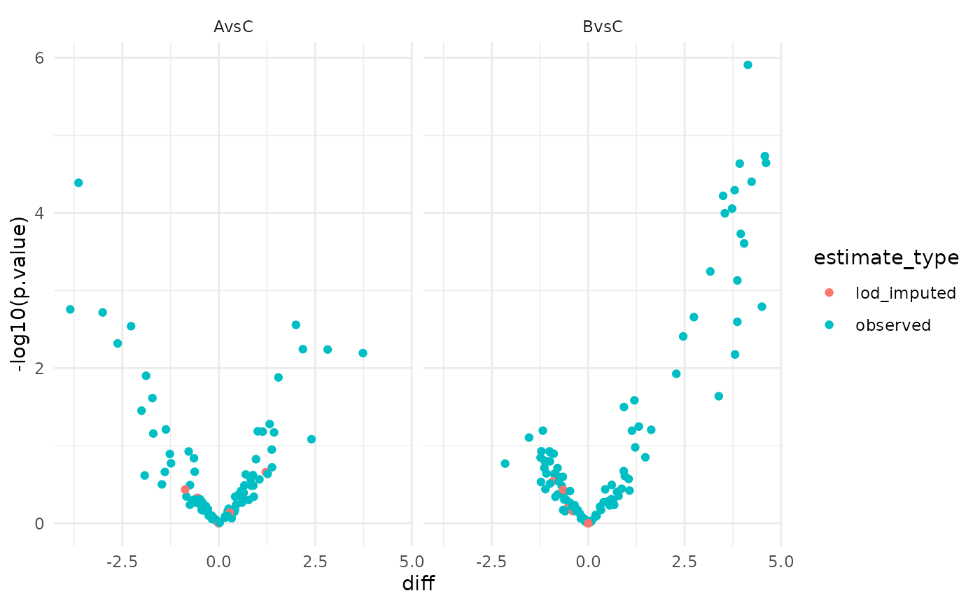
Volcano plot of lm_impute; colour marks the estimates refitted at the LOD.
Other methods
The same refit at the LOD is available with
limma_impute, limma_voom_impute and
rfit_impute. hurdle_nested takes a different
route: it models the intensities and the peptide detection separately
and combines their p-values. The number of estimated protein and
contrast pairs per method:
methods <- c("lm", "lm_impute", "limma", "limma_impute", "rfit", "rfit_impute")
estimated <- vapply(methods, function(m) {
  nrow(build_contrast_analysis(lfq, "~ group_", contrasts, method = m)$get_contrasts())
}, integer(1))
knitr::kable(data.frame(method = methods, estimated = estimated), row.names = FALSE)| method | estimated |
|---|---|
| lm | 194 |
| lm_impute | 200 |
| limma | 192 |
| limma_impute | 200 |
| rfit | 194 |
| rfit_impute | 200 |
The article Comparing modelling methods on one dataset compares them on peptide-level data, including the hurdle model.
Completing the data matrix
impute_from_model() fills every missing cell with the
prediction of its protein model: fitted for proteins fitted
on their observed values, lod_refit for proteins refitted
at the LOD, complete for proteins without missing values.
The filled matrix is useful for heatmaps or clustering. The filled
values carry no noise, so do not use them for further tests.
filled <- impute_from_model(fa_imp$model, lfq)
table(filled$summary$route)
##
## complete fitted lod_refit
## 23 70 7Heatmap before and after
We cluster the proteins once, on the imputed data, and draw both heatmaps with that row order, so each row shows the same protein before and after.
before <- lfq$data_wide(as.matrix = TRUE)
after <- filled$lfqdata$data_wide(as.matrix = TRUE)
row_order <- rownames(after$data)[hclust(dist(t(scale(t(after$data)))))$order]
ht_before <- plot_heatmap(
  before$data, before$annotation, lfq$factor_keys(), lfq$sample_name(),
  na_fraction = 1, row_order = row_order
)
ht_before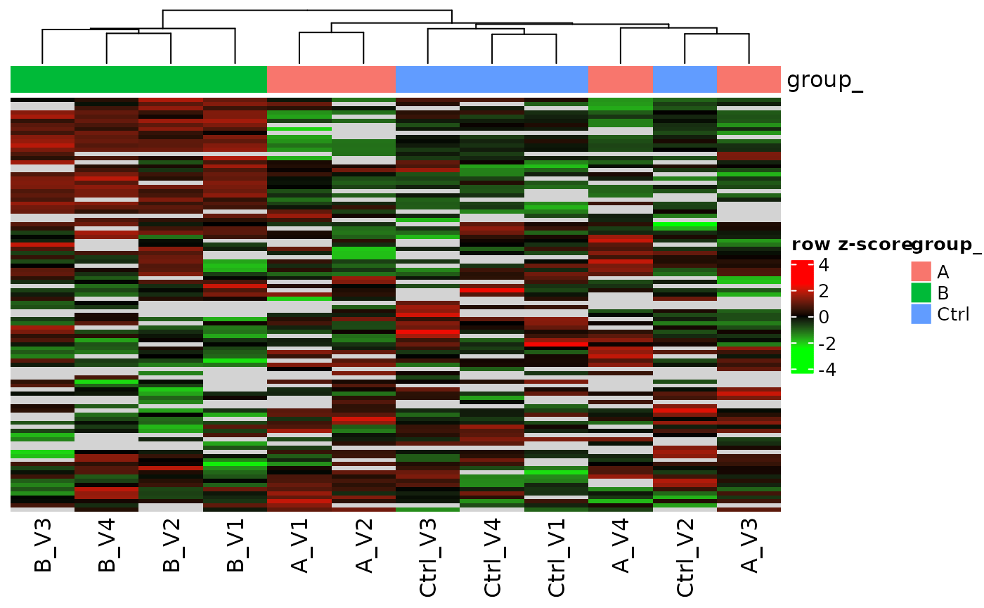
Before imputation: missing cells are grey.
ht_after <- plot_heatmap(
  after$data, after$annotation, lfq$factor_keys(), lfq$sample_name(),
  na_fraction = 1, row_order = row_order
)
ht_after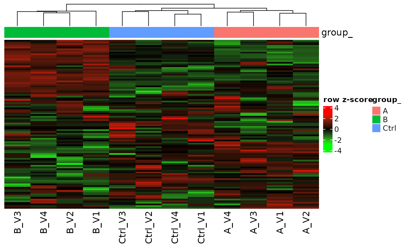
After imputation: every cell holds a value.
PCA before and after
PCA needs complete data. Before imputation it can only use the proteins without missing values; after imputation it uses all proteins.
n_complete <- sum(filled$summary$route == "complete")
gridExtra::grid.arrange(
  lfq$get_Plotter()$pca() +
    ggtitle(paste0("Before imputation: ", n_complete, " complete proteins")),
  filled$lfqdata$get_Plotter()$pca() +
    ggtitle(paste0("After imputation: ", nrow(filled$summary), " proteins")),
  ncol = 1
)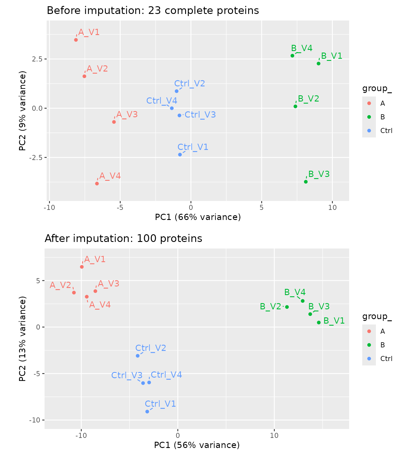
PCA before (top) and after (bottom) imputation.
After imputation the groups separate more cleanly, in the heatmap and in the PCA. Part of that is circular: each filled value is the model’s estimate for its group, so imputation adds the group structure of the model to the data.
Session Info
## R version 4.5.2 (2025-10-31)
## Platform: x86_64-pc-linux-gnu
## Running under: Ubuntu 24.04.5 LTS
##
## Matrix products: default
## BLAS:   /usr/lib/x86_64-linux-gnu/openblas-pthread/libblas.so.3
## LAPACK: /usr/lib/x86_64-linux-gnu/openblas-pthread/libopenblasp-r0.3.26.so;  LAPACK version 3.12.0
##
## locale:
##  [1] LC_CTYPE=C.UTF-8       LC_NUMERIC=C           LC_TIME=C.UTF-8
##  [4] LC_COLLATE=C.UTF-8     LC_MONETARY=C.UTF-8    LC_MESSAGES=C.UTF-8
##  [7] LC_PAPER=C.UTF-8       LC_NAME=C              LC_ADDRESS=C
## [10] LC_TELEPHONE=C         LC_MEASUREMENT=C.UTF-8 LC_IDENTIFICATION=C
##
## time zone: UTC
## tzcode source: system (glibc)
##
## attached base packages:
## [1] stats     graphics  grDevices utils     datasets  methods   base
##
## other attached packages:
## [1] ggplot2_4.0.3  prolfqua_1.9.0
##
## loaded via a namespace (and not attached):
##   [1] Rdpack_2.6.6           gridExtra_2.3.1        rlang_1.3.0
##   [4] magrittr_2.0.5         clue_0.3-68            GetoptLong_1.1.1
##   [7] otel_0.2.0             matrixStats_1.5.0      compiler_4.5.2
##  [10] mgcv_1.9-3             png_0.1-9              systemfonts_1.3.2
##  [13] vctrs_0.7.3            pkgconfig_2.0.3        shape_1.4.6.1
##  [16] crayon_1.5.3           fastmap_1.2.0          backports_1.5.1
##  [19] labeling_0.4.3         utf8_1.2.6             rmarkdown_2.32
##  [22] nloptr_2.2.1           ragg_1.5.2             UpSetR_1.4.1
##  [25] purrr_1.2.2            xfun_0.62              glmnet_5.2
##  [28] jomo_2.7-6             logistf_1.26.1         cachem_1.1.0
##  [31] jsonlite_2.0.0         progress_1.2.3         pan_2.0
##  [34] Rfit_0.27.0            broom_1.0.13           parallel_4.5.2
##  [37] prettyunits_1.2.0      cluster_2.1.8.1        R6_2.6.1
##  [40] bslib_0.12.0           stringi_1.8.9          RColorBrewer_1.1-3
##  [43] limma_3.66.0           boot_1.3-32            rpart_4.1.24
##  [46] jquerylib_0.1.4        Rcpp_1.1.2             iterators_1.0.14
##  [49] knitr_1.52             IRanges_2.44.0         Matrix_1.7-4
##  [52] splines_4.5.2          nnet_7.3-20            tidyselect_1.2.1
##  [55] yaml_2.3.12            doParallel_1.0.17      codetools_0.2-20
##  [58] lattice_0.22-7         tibble_3.3.1           plyr_1.8.9
##  [61] withr_3.0.3            S7_0.2.2               evaluate_1.0.5
##  [64] desc_1.4.3             survival_3.8-3         circlize_0.4.18
##  [67] pillar_1.11.1          mice_3.19.0            foreach_1.5.2
##  [70] stats4_4.5.2           reformulas_0.4.4       plotly_4.12.1
##  [73] generics_0.1.4         S4Vectors_0.48.1       hms_1.1.4
##  [76] scales_1.4.0           minqa_1.2.8            glue_1.8.1
##  [79] tools_4.5.2            data.table_1.18.6.1    lme4_2.1-0
##  [82] forcats_1.0.1          fs_2.1.0               grid_4.5.2
##  [85] tidyr_1.3.2            rbibutils_2.4.1        colorspace_2.1-4
##  [88] nlme_3.1-168           formula.tools_1.7.1    cli_3.6.6
##  [91] textshaping_1.0.5      viridisLite_0.4.3      ComplexHeatmap_2.26.1
##  [94] dplyr_1.2.1            gtable_0.3.6           sass_0.4.10
##  [97] digest_0.6.39          operator.tools_1.6.3.1 BiocGenerics_0.56.0
## [100] ggrepel_0.9.8          rjson_0.2.23           htmlwidgets_1.6.4
## [103] farver_2.1.2           htmltools_0.5.9        pkgdown_2.2.1
## [106] lifecycle_1.0.5        httr_1.4.9             GlobalOptions_0.1.4
## [109] mitml_0.4-5            statmod_1.5.2          MASS_7.3-65