Under the hood: strategy, model and contrasts
Witold E. Wolski
2026-11-20
Source:vignettes/articles/LowLevelAPI.Rmd
LowLevelAPI.RmdPurpose
build_contrast_analysis() chains three steps:
- a strategy says which model to fit per protein,
e.g.
strategy_lm() -
build_model()fits it to every protein and returns aModel -
Contrastscomputes the contrasts from the models;ContrastsModeratedshrinks their variances with the empirical Bayes method
This article runs the steps by hand for the lm method.
Use them to inspect the per-protein models, to change one step, or to
add a new modelling backend. For analyses, use
build_contrast_analysis().
library(prolfqua)
sim <- sim_lfq_data_protein_config(Nprot = 100, seed = 1234)
lfq <- LFQData$new(sim$data, sim$config)
contrasts <- c(AvsC = "group_A - group_Ctrl", BvsC = "group_B - group_Ctrl")
The facade
fa <- build_contrast_analysis(lfq, "~ group_", contrasts, method = "lm")The same, step by step
The lm method weights each protein intensity by its
number of peptides, the column lfq$nr_children_col().
strat <- strategy_lm(paste(lfq$response(), "~ group_"), weights = lfq$nr_children_col())
mod <- build_model(lfq, strat)
contr <- Contrasts$new(mod, contrasts, model_name = "lm")
contr_mod <- ContrastsModerated$new(contr)
Both give the same result:
by_facade <- dplyr::arrange(fa$get_contrasts(), protein_Id, contrast)
by_hand <- dplyr::arrange(contr_mod$get_contrasts(), protein_Id, contrast)
all.equal(by_facade$diff, by_hand$diff)
## [1] TRUE
all.equal(by_facade$p.value, by_hand$p.value)## [1] TRUEThe facade keeps the intermediate objects, so you can also take them
from there: fa$model is the Model,
fa$contrast the moderated contrasts.
Inspecting the models
mod$model_df holds one row per protein with its fitted
model and fit diagnostics.
mod$model_df |>
  dplyr::select(protein_Id, has_model_fit, isSingular, nr_coef_not_NA, sigma, df.residual) |>
  head()
## # A tibble: 6 × 6
## # Groups: protein_Id [6]
## protein_Id has_model_fit isSingular nr_coef_not_NA sigma df.residual
## <chr> <lgl> <lgl> <int> <dbl> <dbl>
## 1 0EfVhX~3967 TRUE FALSE 3 1.40 7
## 2 0m5WN4~6025 TRUE FALSE 3 2.74 8
## 3 0YSKpy~2865 TRUE FALSE 3 1.33 8
## 4 3QLHfm~8938 TRUE FALSE 3 0.907 9
## 5 3QYop0~7543 TRUE FALSE 3 2.38 9
## 6 76k03k~7094 TRUE FALSE 3 2.28 9The analysis of variance per protein, and the distribution of its FDR:
head(mod$get_anova())## # A tibble: 6 × 10
## protein_Id factor Df Sum.Sq Mean.Sq F.value p.value isSingular nr_coef
## <chr> <chr> <int> <dbl> <dbl> <dbl> <dbl> <lgl> <int>
## 1 0EfVhX~3967 group_ 2 20.1 10.1 5.15 0.0421 FALSE 3
## 2 0m5WN4~6025 group_ 2 529. 264. 35.1 0.000109 FALSE 3
## 3 0YSKpy~2865 group_ 2 0.764 0.382 0.217 0.809 FALSE 3
## 4 3QLHfm~8938 group_ 2 5.83 2.92 3.54 0.0733 FALSE 3
## 5 3QYop0~7543 group_ 2 24.9 12.5 2.20 0.167 FALSE 3
## 6 76k03k~7094 group_ 2 9.87 4.93 0.948 0.423 FALSE 3
## # ℹ 1 more variable: FDR <dbl>
mod$anova_histogram("FDR")$plot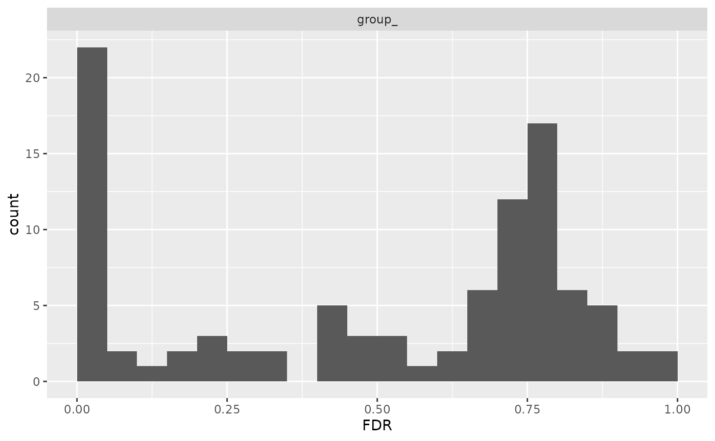
FDR of the per-protein analysis of variance.
The model coefficients:
head(mod$get_coefficients())## # A tibble: 6 × 9
## # Groups: protein_Id [2]
## protein_Id factor Estimate Std..Error df t.value Pr...t.. isSingular
## <chr> <chr> <dbl> <dbl> <int> <dbl> <dbl> <lgl>
## 1 0EfVhX~3967 (Intercept) 22.0 0.494 7 44.5 7.53e-10 FALSE
## 2 0EfVhX~3967 group_B -2.39 0.755 7 -3.17 1.57e- 2 FALSE
## 3 0EfVhX~3967 group_Ctrl -1.37 0.755 7 -1.82 1.12e- 1 FALSE
## 4 0m5WN4~6025 (Intercept) 16.9 0.599 8 28.2 2.68e- 9 FALSE
## 5 0m5WN4~6025 group_B 6.58 0.792 8 8.31 3.32e- 5 FALSE
## 6 0m5WN4~6025 group_Ctrl 3.04 0.792 8 3.84 4.96e- 3 FALSE
## # ℹ 1 more variable: nr_coef <int>From a formula to coefficient weights
setup_analysis() treats configured predictors as
categorical labels. It converts numeric predictors and ordered factors
to character too, so ordered levels and numeric slopes are not retained
by that route. It builds the configured identifiers and retains the
analysis columns; other columns and their attributes are discarded. The
names in config$factors are the predictor names used in the
formula. Method keys, predictor names and contrast names are case
sensitive.
R normally uses treatment coding (options("contrasts")):
an intercept for the reference group and one coefficient per other
level. When predictors are character labels, the first sorted level is
normally the reference. In this small example we explicitly set
Ctrl as the reference to make the coefficients easy to
read:
one_factor <- data.frame(
  group_ = factor(rep(c("Ctrl", "A", "B"), each = 3), levels = c("Ctrl", "A", "B")),
  abundance = c(19.8, 20, 20.2, 21.8, 22, 22.2, 18.8, 19, 19.2)
)
one_model <- lm(abundance ~ group_, data = one_factor)
unique(model.matrix(one_model))
## (Intercept) group_A group_B
## 1 1 0 0
## 4 1 1 0
## 7 1 0 1
coef(one_model)## (Intercept) group_A group_B
## 20 2 -1The coefficient vector is (Intercept),
group_A, group_B: control abundance, A minus
control, and B minus control. linfct_from_model()
represents each group mean as a row of weights on those coefficients.
Internally .model_coeff_matrix() creates the weights for
observed factor combinations and
.coeff_weights_factor_levels() averages them equally within
each factor level. linfct_matrix_contrasts() then evaluates
the named expression using those group rows:
one_means <- linfct_from_model(one_model)$linfct_factors
one_means
## (Intercept) group_A group_B
## group_A 1 1 0
## group_B 1 0 1
## group_Ctrl 1 0 0
one_contrast <- linfct_matrix_contrasts(one_means, c(A_vs_Ctrl = "group_A - group_Ctrl"))
one_contrast
## (Intercept) group_A group_B
## A_vs_Ctrl 0 1 0## A_vs_Ctrl
## 2Here A_vs_Ctrl has weights (0, 1, 0) and
estimates a difference of 2. If A were the reference, the individual
coefficient names and weights would change, but the same contrast of
group means would still estimate A minus control. The contrast strings
refer to group means, which should not be confused with individual
treatment-coded coefficients.
Two factors and their interaction
~ A * B expands to ~ A + B + A:B. With two
levels per factor, its four columns are an intercept, the A effect at
the B reference level, the B effect at the A reference level, and their
interaction. The interaction is the change in the A effect between the
two B levels:
two_factor <- expand.grid(A = c("a0", "a1"), B = c("b0", "b1"), replicate = 1:3)
two_factor$abundance <- 20 + 3 * (two_factor$A == "a1") - 2 * (two_factor$B == "b1") +
  4 * (two_factor$A == "a1" & two_factor$B == "b1") + rep(c(-0.2, 0, 0.2), each = 4)
two_model <- lm(abundance ~ A * B, data = two_factor)
unique(model.matrix(two_model))
## (Intercept) Aa1 Bb1 Aa1:Bb1
## 1 1 0 0 0
## 2 1 1 0 0
## 3 1 0 1 0
## 4 1 1 1 1
coef(two_model)## (Intercept) Aa1 Bb1 Aa1:Bb1
## 20 3 -2 4Cell means include the corresponding intercept, main effects and
interaction. Quote the cell names with backticks because they contain
colons. A main-effect row in linfct_factors averages
equally over the observed cells containing that factor level; a row in
linfct_interactions describes one cell. In this balanced
example, the marginal A difference is 5, the A difference at
b0 is 3, and the difference at b1 is 7:
two_means <- linfct_from_model(two_model)
two_means$linfct_factors
## (Intercept) Aa1 Bb1 Aa1:Bb1
## Aa0 1 0.0 0.5 0.0
## Aa1 1 1.0 0.5 0.5
## Bb0 1 0.5 0.0 0.0
## Bb1 1 0.5 1.0 0.5
two_means$linfct_interactions## (Intercept) Aa1 Bb1 Aa1:Bb1
## Aa0:Bb0 1 0 0 0
## Aa0:Bb1 1 0 1 0
## Aa1:Bb0 1 1 0 0
## Aa1:Bb1 1 1 1 1
two_weights <- linfct_matrix_contrasts(
  linfct_from_model(two_model, as_list = FALSE),
  c(
    A_marginal = "Aa1 - Aa0",
    A_at_b0 = "`Aa1:Bb0` - `Aa0:Bb0`",
    A_at_b1 = "`Aa1:Bb1` - `Aa0:Bb1`",
    A_by_B = "A_at_b1 - A_at_b0"
  )
)
two_weights
## (Intercept) Aa1 Bb1 Aa1:Bb1
## A_marginal 0 1 0 0.5
## A_at_b0 0 1 0 0.0
## A_at_b1 0 1 0 1.0
## A_by_B 0 0 0 1.0## A_marginal A_at_b0 A_at_b1 A_by_B
## 5 3 7 4These helpers assume categorical predictors and the usual intercept-based coding. They do not implement general marginal means for continuous covariates or arbitrary contrast coding. Missing factor combinations can make some rows unestimable; unavailable groups in the contrast expressions are reported by a warning at the low-level interface, and the facade rejects a group absent from the entire dataset.
Without moderation
Contrasts alone gives the unmoderated contrasts, which
the facades do not expose. Moderation stabilises the variances estimated
from few observations:
data.frame(
  contrasts = c("Contrasts", "ContrastsModerated"),
  FDR_lt_0.1 = c(
    sum(contr$get_contrasts()$FDR < 0.1, na.rm = TRUE),
    sum(contr_mod$get_contrasts()$FDR < 0.1, na.rm = TRUE)
  )
)
## contrasts FDR_lt_0.1
## 1 Contrasts 30
## 2 ContrastsModerated 33Changing one step
Replace the strategy to fit another model per protein, e.g. a robust
linear model with strategy_rlm(); the other steps stay the
same.
mod_rlm <- build_model(lfq, strategy_rlm(paste(lfq$response(), "~ group_")))
contr_rlm <- ContrastsModerated$new(Contrasts$new(mod_rlm, contrasts, model_name = "rlm"))
head(contr_rlm$get_contrasts()[, c("protein_Id", "contrast", "diff", "p.value", "FDR")])
## # A tibble: 6 × 5
## protein_Id contrast diff p.value FDR
## <chr> <chr> <dbl> <dbl> <dbl>
## 1 0EfVhX~3967 AvsC 1.27 0.0637 0.328
## 2 0m5WN4~6025 AvsC -3.04 0.0000345 0.000844
## 3 0YSKpy~2865 AvsC 0.144 0.829 0.985
## 4 3QLHfm~8938 AvsC -0.116 0.857 0.985
## 5 3QYop0~7543 AvsC 0.0800 0.911 0.985
## 6 76k03k~7094 AvsC 0.884 0.169 0.519Adding a backend
A facade class wraps the steps of one method.
register_facade() adds it to the registry, after which
build_contrast_analysis(method = ...) finds it.
list_facades() shows the registry:
##  [1] "binomial_firth_nested" "binomial_nested"       "deqms"
##  [4] "deqms_voom"            "firth"                 "hurdle_nested"
##  [7] "limma"                 "limma_impute"          "limma_voom"
## [10] "limma_voom_impute"     "limpa"                 "limpa_nested"
## [13] "lm"                    "lm_impute"             "lmer_nested"
## [16] "rfit"                  "rfit_impute"           "rlm"
## [19] "ropeca_nested"         "ropecaV2_nested"
Session Info
## R version 4.6.2 (2026-10-29)
## Platform: x86_64-pc-linux-gnu
## Running under: Ubuntu 26.04.1 LTS
##
## Matrix products: default
## BLAS:   /usr/lib/x86_64-linux-gnu/openblas-pthread/libblas.so.3
## LAPACK: /usr/lib/x86_64-linux-gnu/openblas-pthread/libopenblasp-r0.3.32.so;  LAPACK version 3.12.0
##
## locale:
##  [1] LC_CTYPE=C.UTF-8       LC_NUMERIC=C           LC_TIME=C.UTF-8
##  [4] LC_COLLATE=C.UTF-8     LC_MONETARY=C.UTF-8    LC_MESSAGES=C.UTF-8
##  [7] LC_PAPER=C.UTF-8       LC_NAME=C              LC_ADDRESS=C
## [10] LC_TELEPHONE=C         LC_MEASUREMENT=C.UTF-8 LC_IDENTIFICATION=C
##
## time zone: UTC
## tzcode source: system (glibc)
##
## attached base packages:
## [1] stats     graphics  grDevices utils     datasets  methods   base
##
## other attached packages:
## [1] prolfqua_1.9.4
##
## loaded via a namespace (and not attached):
##  [1] utf8_1.2.6         sass_0.4.10        generics_0.1.4     tidyr_1.3.2
##  [5] stringi_1.8.9      hms_1.1.4          digest_0.6.39      magrittr_2.0.5
##  [9] evaluate_1.0.5     grid_4.6.2         RColorBrewer_1.1-3 fastmap_1.2.0
## [13] jsonlite_2.0.0     ggrepel_0.9.8      progress_1.2.3     limma_3.68.5
## [17] purrr_1.2.2        scales_1.4.0       textshaping_1.0.5  jquerylib_0.1.4
## [21] cli_3.6.6          rlang_1.3.0        crayon_1.5.3       withr_3.0.3
## [25] cachem_1.1.0       yaml_2.3.12        otel_0.3.0         tools_4.6.2
## [29] dplyr_1.2.1        ggplot2_4.0.4      vctrs_0.7.3        R6_2.6.1
## [33] lifecycle_1.0.5    stringr_1.6.0      fs_2.1.0           htmlwidgets_1.6.4
## [37] MASS_7.3-66        ragg_1.5.2         pkgconfig_2.0.3    desc_1.4.3
## [41] pkgdown_2.2.1      pillar_1.11.1      bslib_0.12.0       gtable_0.3.6
## [45] glue_1.8.1         Rcpp_1.1.2         statmod_1.5.2      systemfonts_1.3.3
## [49] xfun_0.62          tibble_3.3.1       tidyselect_1.2.1   knitr_1.52
## [53] farver_2.1.2       htmltools_0.5.9    labeling_0.4.3     rmarkdown_2.32
## [57] compiler_4.6.2     prettyunits_1.2.0  S7_1.0.0