Contrast Facades with Parallel Designs

Purpose

build_contrast_analysis() provides a common front-end for several contrast backends:

lm — ordinary least-squares linear model fitted per protein, Wald contrasts.
rfit — rank-based robust regression (Rfit::rfit); like lm but resistant to outliers in the response.
limma — linear model with empirical-Bayes moderated variance shrinkage across proteins.
limma_impute — limma with LOD imputation and borrowed per-protein variance for groups with no observations.
limpa — vooma precision-weighted model on DPC-aggregated proteins (requires AggregateLimpa for DPC-based aggregation with standard errors).
lmer — linear mixed-effects model on nested peptide/precursor data, reporting protein-level contrasts.
ropeca — peptide-level fold changes aggregated to protein via ROPECA median + beta-distribution p-values.
lm_missing — lm merged with group-mean substitution for proteins lm cannot estimate (deprecated; prefer lm_impute).
lm_impute — lm that refits failed/singular proteins with LOD imputation and borrowed variance.
deqms — limma plus DEqMS count-dependent variance moderation using peptide counts per protein.
firth — Firth bias-reduced logistic regression on presence/absence (missingness) of aggregated proteins.
firth_nested — Firth logistic regression on peptide-level missingness, reporting protein-level contrasts.

All of them expose the same basic interface: get_contrasts(), get_Plotter(), and to_wide(). All examples below return protein-level contrasts. The important difference is the required input level:

lm, rfit, limma, limma_impute, lm_missing, lm_impute, and deqms require aggregated protein-level data
limpa requires protein-level data from AggregateLimpa (which provides standard errors and observation counts for vooma precision weighting)
lmer and ropeca require lower-level measurements such as peptides nested within proteins, but still report protein-level contrasts
firth can be used with either aggregated protein-level data or nested peptide-level data and still reports protein-level contrasts

This vignette starts from one simulated peptide-level experiment, aggregates it to protein level, and then demonstrates both families of facades separately.

Simulate one experiment

options(prolfqua.vectorize = TRUE)

istar <- sim_lfq_data_peptide_config(Nprot = 80, seed = 42)


lfq_peptide <- LFQData$new(istar$data, istar$config)
lfq_peptide <- lfq_peptide$get_Transformer()$log2()$lfq

lfq_protein <- lfq_peptide$get_Aggregator()$aggregate()

lfq_peptide$hierarchy_keys()

## [1] "protein_Id" "peptide_Id"

lfq_protein$hierarchy_keys()

## [1] "protein_Id"

lfq_protein$nr_children_col()

## [1] "nr_children_protein_Id"

The aggregation step produces protein-level intensities while keeping count metadata in the LFQData object. The DEqMS facade uses lfq_protein$nr_children_col() directly, so no extra count table has to be passed around.

Define contrasts

contrasts <- c(
  "A_vs_Ctrl" = "group_A - group_Ctrl",
  "B_vs_Ctrl" = "group_B - group_Ctrl"
)

Two contrasts let us see how each backend handles multiple comparisons and how FDR correction propagates across contrasts.

Protein-input facades

The following facades require aggregated input, which in practice means lfqdata$subject_id() must match lfqdata$hierarchy_keys(). firth is included here on purpose because it can be fitted directly on aggregated protein input.

fa_lm <- build_contrast_analysis(
  lfq_protein,
  "~ group_",
  contrasts,
  method = "lm"
)

fa_rfit <- build_contrast_analysis(
  lfq_protein,
  "~ group_",
  contrasts,
  method = "rfit"
)

fa_limma <- build_contrast_analysis(
  lfq_protein,
  "~ group_",
  contrasts,
  method = "limma"
)

fa_limma_impute <- build_contrast_analysis(
  lfq_protein,
  "~ group_",
  contrasts,
  method = "limma_impute"
)

fa_lm_missing <- build_contrast_analysis(
  lfq_protein,
  "~ group_",
  contrasts,
  method = "lm_missing"
)

fa_deqms <- build_contrast_analysis(
  lfq_protein,
  "~ group_",
  contrasts,
  method = "deqms"
)

fa_lm_impute <- build_contrast_analysis(
  lfq_protein,
  "~ group_",
  contrasts,
  method = "lm_impute"
)

fa_firth_protein <- build_contrast_analysis(
  lfq_protein,
  "~ group_",
  contrasts,
  method = "firth"
)

limpa facade (DPC-based aggregation)

The limpa facade is different from the other protein-level facades: it requires its own aggregation step via AggregateLimpa, which uses limpa’s Detection Probability Curve (DPC) to aggregate peptides to proteins while producing per-protein, per-sample standard errors. These SEs feed into a bivariate vooma variance model for precision weighting.

lfq_limpa <- AggregateLimpa$new(lfq_peptide, "protein")$aggregate()

fa_limpa <- build_contrast_analysis(
  lfq_limpa,
  "~ group_",
  contrasts,
  method = "limpa"
)

Because all protein-input facades share the same interface and report protein-level contrasts, their outputs can be combined directly.

# Proteins missing in the baseline lm facade (used to flag rescued proteins)
lm_missing_ids <- fa_lm$get_missing() |>
  dplyr::select(protein_Id, contrast) |>
  dplyr::mutate(rescued = TRUE)

results_limpa <- if (requireNamespace("limpa", quietly = TRUE)) {
  fa_limpa$get_contrasts()
} else {
  data.frame()
}

results_protein <- bind_rows(
  fa_lm$get_contrasts(),
  fa_rfit$get_contrasts(),
  fa_limma$get_contrasts(),
  fa_limma_impute$get_contrasts(),
  fa_lm_missing$get_contrasts(),
  fa_lm_impute$get_contrasts(),
  fa_deqms$get_contrasts(),
  fa_firth_protein$get_contrasts(),
  results_limpa
) |>
  dplyr::select(dplyr::any_of(c(
    "facade", "modelName", "protein_Id", "contrast", "avgAbd", "diff", "FDR",
    "statistic", "std.error", "df", "p.value", "conf.low", "conf.high",
    "sigma"
  ))) |>
  dplyr::left_join(lm_missing_ids, by = c("protein_Id", "contrast")) |>
  dplyr::mutate(
    rescued = dplyr::coalesce(rescued, FALSE),
    significant = FDR < 0.1 & abs(diff) > 0.5
  )

results_protein |>
  dplyr::count(facade, name = "n_results")

## # A tibble: 9 × 2
##   facade       n_results
##   <chr>            <int>
## 1 deqms              157
## 2 firth              160
## 3 limma              155
## 4 limma_impute       160
## 5 limpa              160
## 6 lm                 157
## 7 lm_impute          160
## 8 lm_missing         160
## 9 rfit               157

For facades that combine several underlying result types, such as lm_missing, the modelName column still tells you where individual rows came from.

results_protein |>
  dplyr::count(facade, contrast, modelName, name = "n_results")

## # A tibble: 24 × 4
##    facade       contrast  modelName      n_results
##    <chr>        <chr>     <chr>              <int>
##  1 deqms        A_vs_Ctrl WaldTest_DEqMS        78
##  2 deqms        B_vs_Ctrl WaldTest_DEqMS        79
##  3 firth        A_vs_Ctrl WaldTestFirth         80
##  4 firth        B_vs_Ctrl WaldTestFirth         80
##  5 limma        A_vs_Ctrl limma                 78
##  6 limma        B_vs_Ctrl limma                 77
##  7 limma_impute A_vs_Ctrl limma                 77
##  8 limma_impute A_vs_Ctrl limma_imputed          3
##  9 limma_impute B_vs_Ctrl limma                 77
## 10 limma_impute B_vs_Ctrl limma_imputed          3
## # ℹ 14 more rows

Protein-level volcano comparison

Standard facades

standard_facades <- c("lm", "rfit", "limma", "deqms")
results_standard <- results_protein |>
  dplyr::filter(facade %in% standard_facades)

ggplot(results_standard, aes(x = diff, y = -log10(p.value), color = significant)) +
  geom_point(alpha = 0.6, size = 1.5) +
  facet_grid(contrast ~ facade, scales = "free_y") +
  geom_vline(xintercept = c(-0.5, 0.5), linetype = "dashed", color = "grey60") +
  geom_hline(yintercept = -log10(0.1), linetype = "dashed", color = "grey60") +
  scale_color_manual(values = c(`TRUE` = "firebrick", `FALSE` = "grey70")) +
  labs(x = "log2 fold change", y = "-log10(p.value)", color = "FDR < 0.1\nand |diff| > 0.5") +
  theme_minimal(base_size = 12)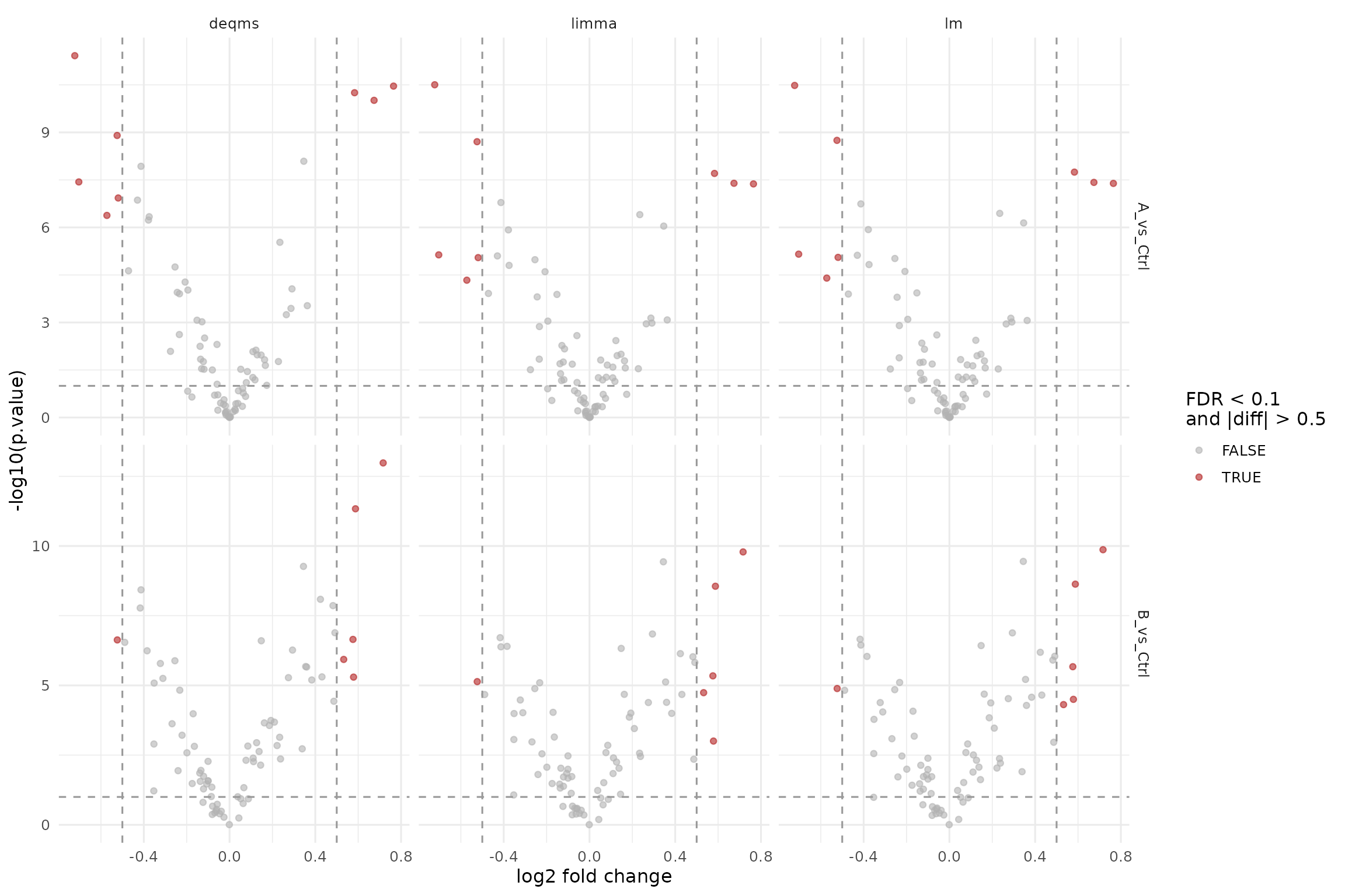

Volcano plots for the standard protein-level facades (lm, rfit, limma, deqms).

Imputation and missingness facades

Rescued proteins (missing in plain lm) are shown as large red diamonds so they stand out clearly. This group includes the LOD imputation facades (lm_missing, lm_impute, limma_impute) and the firth logistic regression facade which models missingness directly.

impute_facades <- c("lm_missing", "lm_impute", "limma_impute", "firth")
results_impute <- results_protein |>
  dplyr::filter(facade %in% impute_facades) |>
  dplyr::mutate(facade = factor(facade, levels = impute_facades))

ggplot(results_impute, aes(x = diff, y = -log10(p.value))) +
  geom_point(data = dplyr::filter(results_impute, !rescued),
             aes(color = significant), alpha = 0.5, size = 1.2) +
  geom_point(data = dplyr::filter(results_impute, rescued),
             color = "red", shape = 18, size = 5, alpha = 1) +
  facet_grid(contrast ~ facade, scales = "free_y") +
  geom_vline(xintercept = c(-0.5, 0.5), linetype = "dashed", color = "grey60") +
  geom_hline(yintercept = -log10(0.1), linetype = "dashed", color = "grey60") +
  scale_color_manual(values = c(`TRUE` = "firebrick", `FALSE` = "grey70")) +
  labs(x = "log2 fold change", y = "-log10(p.value)", color = "FDR < 0.1\nand |diff| > 0.5") +
  theme_minimal(base_size = 12)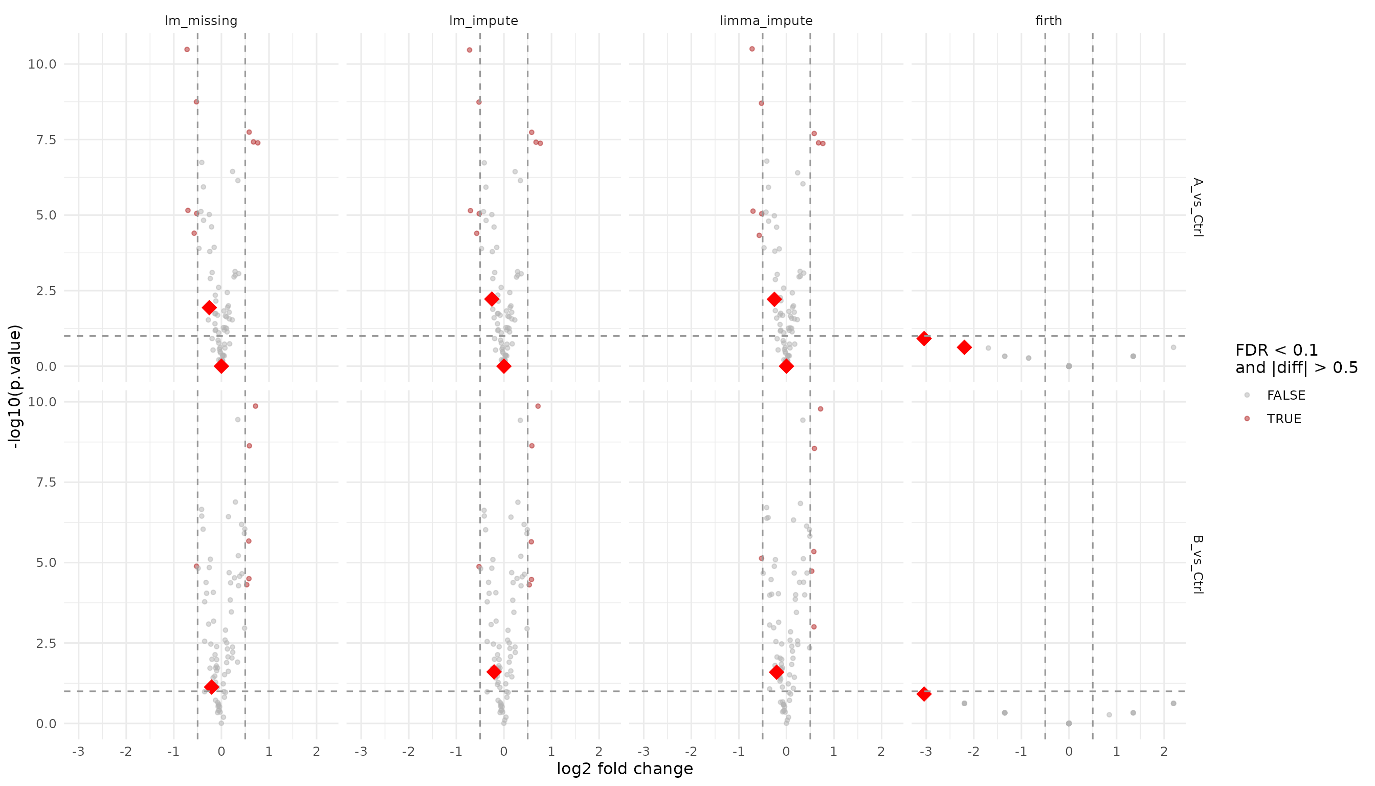

Volcano plots for the imputation and missingness facades. Large red diamonds mark proteins rescued (missing in plain lm).

Looking at the strongest protein-level hits

results_protein |>
  dplyr::group_by(facade, contrast) |>
  dplyr::slice_min(order_by = p.value, n = 5, with_ties = FALSE) |>
  dplyr::ungroup() |>
  dplyr::select(facade, contrast, modelName, protein_Id, diff, p.value, FDR)

## # A tibble: 90 × 7
##    facade contrast  modelName      protein_Id    diff  p.value      FDR
##    <chr>  <chr>     <chr>          <chr>        <dbl>    <dbl>    <dbl>
##  1 deqms  A_vs_Ctrl WaldTest_DEqMS Zci7Jw~7064 -0.722 3.79e-12 2.96e-10
##  2 deqms  A_vs_Ctrl WaldTest_DEqMS 6TevMr~7550  0.765 3.46e-11 1.35e- 9
##  3 deqms  A_vs_Ctrl WaldTest_DEqMS 4Y4DYT~0927  0.583 5.59e-11 1.45e- 9
##  4 deqms  A_vs_Ctrl WaldTest_DEqMS 0CubNR~0890  0.674 9.73e-11 1.90e- 9
##  5 deqms  A_vs_Ctrl WaldTest_DEqMS KVkccD~1805 -0.524 1.25e- 9 1.95e- 8
##  6 deqms  B_vs_Ctrl WaldTest_DEqMS fylZqB~3883  0.717 1.05e-13 8.28e-12
##  7 deqms  B_vs_Ctrl WaldTest_DEqMS XxJoJB~7286  0.587 4.63e-12 1.83e-10
##  8 deqms  B_vs_Ctrl WaldTest_DEqMS f0Cvvj~6658  0.345 5.39e-10 1.42e- 8
##  9 deqms  B_vs_Ctrl WaldTest_DEqMS TR3Ksv~1492 -0.413 3.73e- 9 7.37e- 8
## 10 deqms  B_vs_Ctrl WaldTest_DEqMS 4Y4DYT~0927  0.424 8.16e- 9 1.29e- 7
## # ℹ 80 more rows

Proteins that could not be estimated

Every facade has a get_missing() method that returns the protein × contrast pairs present in the input data but absent from get_contrasts(). This makes it easy to see which proteins each method fails on and to compare coverage.

missing_limpa <- if (requireNamespace("limpa", quietly = TRUE)) {
  fa_limpa$get_missing() |> dplyr::mutate(facade = "limpa")
} else {
  data.frame()
}

missing_all <- dplyr::bind_rows(
  fa_lm$get_missing() |> dplyr::mutate(facade = "lm"),
  fa_limma$get_missing() |> dplyr::mutate(facade = "limma"),
  fa_limma_impute$get_missing() |> dplyr::mutate(facade = "limma_impute"),
  fa_lm_missing$get_missing() |> dplyr::mutate(facade = "lm_missing"),
  fa_lm_impute$get_missing() |> dplyr::mutate(facade = "lm_impute"),
  fa_deqms$get_missing() |> dplyr::mutate(facade = "deqms"),
  fa_firth_protein$get_missing() |> dplyr::mutate(facade = "firth"),
  missing_limpa
)

missing_all |>
  dplyr::count(facade, contrast, name = "n_missing") |>
  knitr::kable(caption = "Number of missing protein × contrast pairs per facade")

Number of missing protein × contrast pairs per facade
facade	contrast	n_missing
deqms	A_vs_Ctrl	2
deqms	B_vs_Ctrl	1
limma	A_vs_Ctrl	2
limma	B_vs_Ctrl	3
lm	A_vs_Ctrl	2
lm	B_vs_Ctrl	1

Per-sample intensities of the missing proteins

missing_proteins <- unique(missing_all$protein_Id)

if (length(missing_proteins) > 0) {
  lfq_protein$data_long() |>
    dplyr::filter(protein_Id %in% missing_proteins) |>
    dplyr::select(protein_Id, sampleName,
                  !!rlang::sym(lfq_protein$response())) |>
    tidyr::pivot_wider(names_from = sampleName,
                       values_from = !!rlang::sym(lfq_protein$response())) |>
    knitr::kable(digits = 2, caption = "Per-sample intensities of proteins that could not be estimated")
}

Per-sample intensities of proteins that could not be estimated
protein_Id	A_V1	A_V2	A_V3	A_V4	B_V1	B_V2	B_V3	B_V4	Ctrl_V1	Ctrl_V2	Ctrl_V3	Ctrl_V4
8mS8sK~0150	NA	NA	NA	NA	3.85	NA	NA	3.76	NA	NA	3.37	3.55
DTCi0N~0734	NA	NA	NA	NA	NA	4.37	4.35	4.28	NA	4.06	4.07	4.21
OrL0ux~1369	NA	NA	NA	3.78	NA	NA	NA	NA	4.12	4.05	NA	3.98

The missing cells (NA) explain why these proteins cannot be estimated — they lack observations in one or more groups. The lm_missing facade fills in these gaps via group-mean imputation, while lm_impute and limma_impute re-fit after imputing individual values with the LOD and borrowing covariance from successful fits. These should have fewer missing proteins than plain lm or limma.

Estimates for the missing proteins from `lm_missing` and `lm_impute`

For proteins that plain lm could not estimate, the imputation-based facades can still produce contrast results. The table below shows these rescued estimates side by side.

lm_missing_proteins <- fa_lm$get_missing()$protein_Id |> unique()

if (length(lm_missing_proteins) > 0) {
  rescued <- results_protein |>
    dplyr::filter(
      protein_Id %in% lm_missing_proteins,
      facade %in% c("lm_missing", "lm_impute", "limma_impute", "limpa")
    ) |>
    dplyr::arrange(protein_Id, contrast, facade)

  rescued |>
    knitr::kable(
      digits = 3,
      caption = "Contrast estimates from lm_missing, lm_impute, and limma_impute for proteins that plain lm could not estimate"
    )
} else {
  cat("All proteins were estimable by plain lm — no rescued estimates to show.")
}

Contrast estimates from lm_missing, lm_impute, and limma_impute for proteins that plain lm could not estimate
facade	modelName	protein_Id	contrast	avgAbd	diff	FDR	statistic	std.error	df	p.value	conf.low	conf.high	sigma	rescued	significant
limma_impute	limma_imputed	8mS8sK~0150	A_vs_Ctrl	3.776	0.000	1.000	0.000	0.063	4.468	1.000	-0.167	0.167	0.089	TRUE	FALSE
limpa	limpa	8mS8sK~0150	A_vs_Ctrl	2.798	-0.615	0.226	-1.435	0.429	30.965	0.161	-1.489	0.259	0.965	TRUE	FALSE
lm_impute	WaldTest_moderated_imputed	8mS8sK~0150	A_vs_Ctrl	3.776	0.000	1.000	0.000	0.065	4.310	1.000	-0.234	0.234	0.087	TRUE	FALSE
lm_missing	groupAverage	8mS8sK~0150	A_vs_Ctrl	3.697	0.000	1.000	0.000	0.102	2.000	1.000	-0.437	0.437	0.102	TRUE	FALSE
limma_impute	limma_imputed	8mS8sK~0150	B_vs_Ctrl	3.784	0.018	0.803	0.279	0.063	4.468	0.792	-0.150	0.185	0.089	FALSE	FALSE
limpa	limpa	8mS8sK~0150	B_vs_Ctrl	3.245	0.279	0.578	0.662	0.422	30.965	0.513	-0.581	1.140	0.965	FALSE	FALSE
lm_impute	WaldTest_moderated_imputed	8mS8sK~0150	B_vs_Ctrl	3.784	0.018	0.798	0.286	0.065	4.310	0.788	-0.217	0.252	0.087	FALSE	FALSE
lm_missing	WaldTest_moderated	8mS8sK~0150	B_vs_Ctrl	3.632	0.339	0.020	3.690	0.102	5.377	0.012	0.108	0.570	0.092	FALSE	FALSE
limma_impute	limma_imputed	DTCi0N~0734	A_vs_Ctrl	3.902	-0.253	0.017	-3.996	0.063	6.468	0.006	-0.405	-0.101	0.090	TRUE	FALSE
limpa	limpa	DTCi0N~0734	A_vs_Ctrl	3.550	-0.982	0.020	-2.714	0.362	30.965	0.011	-1.719	-0.244	0.991	TRUE	TRUE
lm_impute	WaldTest_moderated_imputed	DTCi0N~0734	A_vs_Ctrl	3.902	-0.253	0.017	-4.057	0.065	6.310	0.006	-0.467	-0.040	0.088	TRUE	FALSE
lm_missing	groupAverage	DTCi0N~0734	A_vs_Ctrl	3.902	-0.253	0.032	-4.417	0.057	4.000	0.012	-0.412	-0.094	0.070	TRUE	FALSE
limma_impute	limma_imputed	DTCi0N~0734	B_vs_Ctrl	4.112	0.166	0.051	2.626	0.063	6.468	0.037	0.014	0.319	0.090	FALSE	FALSE
limpa	limpa	DTCi0N~0734	B_vs_Ctrl	4.145	0.208	0.619	0.581	0.358	30.965	0.565	-0.522	0.939	0.991	FALSE	FALSE
lm_impute	WaldTest_moderated_imputed	DTCi0N~0734	B_vs_Ctrl	4.112	0.166	0.049	2.665	0.065	6.310	0.035	-0.047	0.380	0.088	FALSE	FALSE
lm_missing	WaldTest_moderated	DTCi0N~0734	B_vs_Ctrl	4.224	0.222	0.016	3.499	0.057	7.377	0.009	0.040	0.403	0.078	FALSE	FALSE
limma_impute	limma_imputed	OrL0ux~1369	A_vs_Ctrl	3.879	-0.207	0.050	-3.293	0.063	4.468	0.026	-0.374	-0.039	0.089	FALSE	FALSE
limpa	limpa	OrL0ux~1369	A_vs_Ctrl	3.497	-0.881	0.025	-2.630	0.335	30.965	0.013	-1.563	-0.198	0.960	FALSE	TRUE
lm_impute	WaldTest_moderated_imputed	OrL0ux~1369	A_vs_Ctrl	3.879	-0.207	0.049	-3.369	0.065	4.310	0.025	-0.441	0.028	0.087	FALSE	FALSE
lm_missing	WaldTest_moderated	OrL0ux~1369	A_vs_Ctrl	3.913	-0.276	0.055	-2.951	0.084	5.340	0.029	-0.480	-0.072	0.081	FALSE	FALSE
limma_impute	limma_imputed	OrL0ux~1369	B_vs_Ctrl	3.879	-0.207	0.038	-3.293	0.063	4.468	0.026	-0.374	-0.039	0.089	TRUE	FALSE
limpa	limpa	OrL0ux~1369	B_vs_Ctrl	3.297	-1.281	0.006	-3.200	0.400	30.965	0.003	-2.097	-0.464	0.960	TRUE	TRUE
lm_impute	WaldTest_moderated_imputed	OrL0ux~1369	B_vs_Ctrl	3.879	-0.207	0.036	-3.369	0.065	4.310	0.025	-0.441	0.028	0.087	TRUE	FALSE
lm_missing	groupAverage	OrL0ux~1369	B_vs_Ctrl	3.879	-0.207	0.094	-3.473	0.060	2.000	0.074	-0.463	0.049	0.073	TRUE	FALSE

Peptide-input facades

The peptide-input facades take peptide/precursor-level LFQData and return protein-level contrasts. They are defined in R/ContrastsChildToParentFacades.R and use the *_nested method keys: lmer_nested, ropeca_nested, firth_nested, and limpa_nested. firth_nested is the peptide-input counterpart of the protein-input firth shown above.

fa_lmer <- build_contrast_analysis(
  lfq_peptide,
  "~ group_ + (1 | peptide_Id) + (1 | sampleName)",
  contrasts,
  method = "lmer_nested"
)

fa_ropeca <- build_contrast_analysis(
  lfq_peptide,
  "~ group_",
  contrasts,
  method = "ropeca_nested"
)

fa_firth_peptide <- build_contrast_analysis(
  lfq_peptide,
  "~ group_",
  contrasts,
  method = "firth_nested"
)

ropeca_nested aggregates peptide evidence back to proteins, whereas lmer_nested models the nested peptide structure directly before reporting protein-level contrasts. firth_nested also reports protein-level contrasts: proteins with exactly one peptide are fitted without an added peptide term, while proteins with multiple peptides are fitted with the lowest hierarchy key added internally.

results_peptide <- bind_rows(
  fa_lmer$get_contrasts(),
  fa_ropeca$get_contrasts(),
  fa_firth_peptide$get_contrasts()
) |>
  dplyr::select(dplyr::any_of(c(
    "facade", "modelName", "protein_Id", "contrast", "avgAbd", "diff", "FDR",
    "statistic", "std.error", "df", "p.value", "conf.low", "conf.high",
    "sigma"
  ))) |>
  dplyr::mutate(
    significant = FDR < 0.1 & abs(diff) > 0.5
  )

results_peptide |>
  dplyr::count(facade, name = "n_results")

## # A tibble: 3 × 2
##   facade        n_results
##   <chr>             <int>
## 1 firth_nested        160
## 2 lmer_nested         102
## 3 ropeca_nested       157

ggplot(results_peptide, aes(x = diff, y = -log10(p.value), color = significant)) +
  geom_point(alpha = 0.6, size = 1.2) +
  facet_grid(contrast ~ facade, scales = "free_y") +
  geom_vline(xintercept = c(-0.5, 0.5), linetype = "dashed", color = "grey60") +
  geom_hline(yintercept = -log10(0.1), linetype = "dashed", color = "grey60") +
  scale_color_manual(values = c(`TRUE` = "firebrick", `FALSE` = "grey70")) +
  labs(
    x = "log2 fold change",
    y = "-log10(p.value)",
    color = "FDR < 0.1\nand |diff| > 0.5"
  ) +
  theme_minimal(base_size = 12)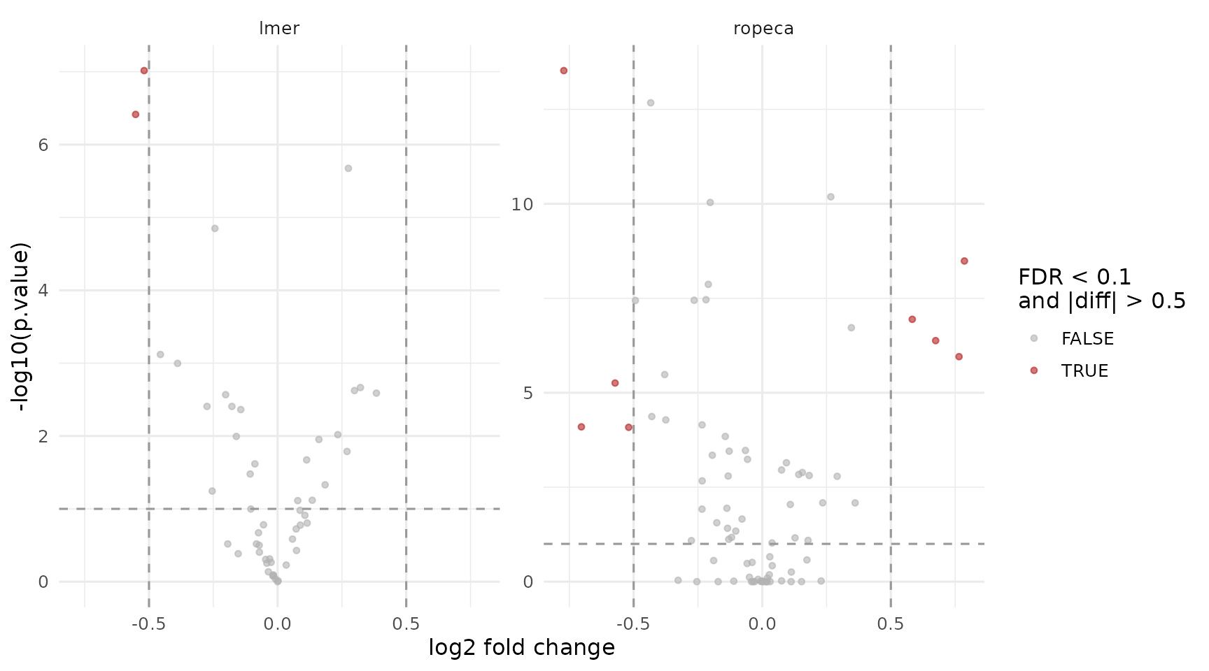

Volcano plots for the peptide-level facades. Rows are contrasts, columns are backends.

Remarks

The facades make it easy to benchmark alternative contrast backends without rewriting the analysis pipeline:

the protein-level facades now enforce aggregation before modelling
the limpa facade uses its own DPC-based aggregation (AggregateLimpa) which produces standard errors propagated into vooma precision weights
the peptide-level facades now explicitly require lower-level hierarchy below the analysis subject
the shared facade API still makes it straightforward to compare methods once the data level is chosen consistently

The results are comparable at the API level, but the comparison is only meaningful when methods using the same biological unit are plotted together.

Session Info

sessionInfo()

## R version 4.5.2 (2025-10-31)
## Platform: x86_64-pc-linux-gnu
## Running under: Ubuntu 24.04.4 LTS
## 
## Matrix products: default
## BLAS:   /usr/lib/x86_64-linux-gnu/openblas-pthread/libblas.so.3 
## LAPACK: /usr/lib/x86_64-linux-gnu/openblas-pthread/libopenblasp-r0.3.26.so;  LAPACK version 3.12.0
## 
## locale:
##  [1] LC_CTYPE=C.UTF-8       LC_NUMERIC=C           LC_TIME=C.UTF-8       
##  [4] LC_COLLATE=C.UTF-8     LC_MONETARY=C.UTF-8    LC_MESSAGES=C.UTF-8   
##  [7] LC_PAPER=C.UTF-8       LC_NAME=C              LC_ADDRESS=C          
## [10] LC_TELEPHONE=C         LC_MEASUREMENT=C.UTF-8 LC_IDENTIFICATION=C   
## 
## time zone: UTC
## tzcode source: system (glibc)
## 
## attached base packages:
## [1] stats     graphics  grDevices utils     datasets  methods   base     
## 
## other attached packages:
## [1] ggplot2_4.0.3  dplyr_1.2.1    prolfqua_1.6.3
## 
## loaded via a namespace (and not attached):
##   [1] Rdpack_2.6.6           gridExtra_2.3          rlang_1.2.0           
##   [4] magrittr_2.0.5         clue_0.3-68            GetoptLong_1.1.1      
##   [7] otel_0.2.0             matrixStats_1.5.0      compiler_4.5.2        
##  [10] mgcv_1.9-3             png_0.1-9              systemfonts_1.3.2     
##  [13] vctrs_0.7.3            pkgconfig_2.0.3        shape_1.4.6.1         
##  [16] crayon_1.5.3           fastmap_1.2.0          backports_1.5.1       
##  [19] labeling_0.4.3         utf8_1.2.6             rmarkdown_2.31        
##  [22] nloptr_2.2.1           ragg_1.5.2             UpSetR_1.4.1          
##  [25] purrr_1.2.2            xfun_0.59              glmnet_5.0            
##  [28] jomo_2.7-6             logistf_1.26.1         cachem_1.1.0          
##  [31] jsonlite_2.0.0         progress_1.2.3         pan_1.9               
##  [34] Rfit_0.27.0            prettyunits_1.2.0      broom_1.0.13          
##  [37] parallel_4.5.2         cluster_2.1.8.1        R6_2.6.1              
##  [40] bslib_0.11.0           stringi_1.8.7          RColorBrewer_1.1-3    
##  [43] limma_3.66.0           boot_1.3-32            rpart_4.1.24          
##  [46] numDeriv_2016.8-1.1    jquerylib_0.1.4        Rcpp_1.1.1-1.1        
##  [49] iterators_1.0.14       knitr_1.51             IRanges_2.44.0        
##  [52] Matrix_1.7-4           splines_4.5.2          nnet_7.3-20           
##  [55] tidyselect_1.2.1       yaml_2.3.12            doParallel_1.0.17     
##  [58] codetools_0.2-20       lmerTest_3.2-1         lattice_0.22-7        
##  [61] tibble_3.3.1           plyr_1.8.9             withr_3.0.3           
##  [64] S7_0.2.2               evaluate_1.0.5         desc_1.4.3            
##  [67] survival_3.8-3         circlize_0.4.18        pillar_1.11.1         
##  [70] mice_3.19.0            foreach_1.5.2          stats4_4.5.2          
##  [73] reformulas_0.4.4       plotly_4.12.0          generics_0.1.4        
##  [76] hms_1.1.4              S4Vectors_0.48.1       scales_1.4.0          
##  [79] minqa_1.2.8            glue_1.8.1             lazyeval_0.2.3        
##  [82] tools_4.5.2            data.table_1.18.4      lme4_2.0-1            
##  [85] forcats_1.0.1          fs_2.1.0               grid_4.5.2            
##  [88] limpa_1.2.5            tidyr_1.3.2            rbibutils_2.4.1       
##  [91] colorspace_2.1-2       nlme_3.1-168           formula.tools_1.7.1   
##  [94] cli_3.6.6              textshaping_1.0.5      viridisLite_0.4.3     
##  [97] ComplexHeatmap_2.26.1  gtable_0.3.6           sass_0.4.10           
## [100] digest_0.6.39          operator.tools_1.6.3.1 BiocGenerics_0.56.0   
## [103] ggrepel_0.9.8          rjson_0.2.23           htmlwidgets_1.6.4     
## [106] farver_2.1.2           htmltools_0.5.9        pkgdown_2.2.0         
## [109] lifecycle_1.0.5        httr_1.4.8             GlobalOptions_0.1.4   
## [112] mitml_0.4-5            statmod_1.5.2          MASS_7.3-65

Witold E. Wolski

2026-06-23

Purpose

Simulate one experiment

Define contrasts

Protein-input facades

limpa facade (DPC-based aggregation)

Protein-level volcano comparison

Standard facades

Imputation and missingness facades

Looking at the strongest protein-level hits

Proteins that could not be estimated

Per-sample intensities of the missing proteins

Estimates for the missing proteins from `lm_missing` and `lm_impute`

Peptide-input facades

Remarks

Session Info

Contrast Facades with Parallel Designs

Witold E. Wolski

2026-06-23

Purpose

Simulate one experiment

Define contrasts

Protein-input facades

limpa facade (DPC-based aggregation)

Protein-level volcano comparison

Standard facades

Imputation and missingness facades

Looking at the strongest protein-level hits

Proteins that could not be estimated

Per-sample intensities of the missing proteins

Estimates for the missing proteins from lm_missing and lm_impute

Peptide-input facades

Remarks

Session Info

Estimates for the missing proteins from `lm_missing` and `lm_impute`