Using limpa Directly on prolfqua Simulated Data

This vignette demonstrates how to use the limpa package directly (without prolfqua wrappers) on peptide-level data simulated with prolfqua. Three analyses are shown:

Baseline: limma with NAs — standard limma on protein-level medpolish-aggregated data (NAs dropped)
limpa peptide-level — differential expression at the peptide level (no protein aggregation)
limpa protein-level — limpa aggregates peptides to proteins via dpcQuant(), then tests for DE

Setup and Data Simulation

library(prolfqua)
library(limpa)
library(limma)

Simulate peptide-level data with 3 groups (Ctrl, A, B), 5 replicates per group, and 50 proteins with realistic missing values.

sim <- prolfqua::sim_lfq_data_peptide_config(
  Nprot = 50, N = 5, with_missing = TRUE, seed = 1234
)
lfqdata <- prolfqua::LFQData$new(sim$data, sim$config)

Log2-transform and pivot to a wide matrix (peptides x samples) for limpa.

lfqdata <- lfqdata$get_Transformer()$log2()$lfq
wide <- lfqdata$to_wide(as.matrix = TRUE)

expr_matrix <- wide$data
annotation <- wide$annotation
rowdata <- wide$rowdata

cat("Matrix dimensions:", nrow(expr_matrix), "peptides x", ncol(expr_matrix), "samples\n")

## Matrix dimensions: 152 peptides x 15 samples

cat("Missing values:", sum(is.na(expr_matrix)), "of", length(expr_matrix),
    sprintf("(%.1f%%)\n", 100 * sum(is.na(expr_matrix)) / length(expr_matrix)))

## Missing values: 278 of 2280 (12.2%)

cat("Proteins:", length(unique(rowdata$protein_Id)), "\n")

## Proteins: 50

Design Matrix and Contrasts

All analyses below use the same design matrix: a cell-means model with three groups.

group <- factor(annotation$group_, levels = c("Ctrl", "A", "B"))
design <- stats::model.matrix(~ 0 + group)
colnames(design) <- levels(group)

cont_matrix <- limma::makeContrasts(
  A_vs_Ctrl = A - Ctrl,
  B_vs_Ctrl = B - Ctrl,
  levels = design
)

Baseline: Standard limma Analysis (no limpa)

As a baseline, aggregate peptides to proteins using prolfqua’s medpolish aggregator, then run a plain limma::lmFit() + eBayes() analysis. NAs are simply ignored by limma.

lfqdata_protein <- lfqdata$get_Aggregator()$aggregate()
wide_prot <- lfqdata_protein$to_wide(as.matrix = TRUE)
expr_protein_baseline <- wide_prot$data

cat("Protein matrix:", nrow(expr_protein_baseline), "proteins x",
    ncol(expr_protein_baseline), "samples\n")

## Protein matrix: 50 proteins x 15 samples

cat("NAs in protein matrix:", sum(is.na(expr_protein_baseline)), "\n")

## NAs in protein matrix: 48

Fit limma. lmFit handles NAs by fitting each protein on its available samples only.

fit_baseline <- limma::lmFit(expr_protein_baseline, design)
fit_baseline <- limma::contrasts.fit(fit_baseline, cont_matrix)
fit_baseline <- limma::eBayes(fit_baseline)

results_baseline_A <- limma::topTable(fit_baseline, coef = "A_vs_Ctrl", number = Inf, sort.by = "none")
cat("Baseline limma — A vs Ctrl: ", sum(results_baseline_A$adj.P.Val < 0.05),
    "significant proteins at FDR < 0.05\n")

## Baseline limma — A vs Ctrl:  40 significant proteins at FDR < 0.05

results_baseline_B <- limma::topTable(fit_baseline, coef = "B_vs_Ctrl", number = Inf, sort.by = "none")
cat("Baseline limma — B vs Ctrl: ", sum(results_baseline_B$adj.P.Val < 0.05),
    "significant proteins at FDR < 0.05\n")

## Baseline limma — B vs Ctrl:  36 significant proteins at FDR < 0.05

Estimate the Detection Probability Curve (DPC)

The DPC models the probability of observing a peptide as a logit-linear function of its intensity: logit P(detected) = beta0 + beta1 * intensity. This is a global parameter estimated once from the entire peptide-level dataset.

beta1 (slope) controls the strength of intensity-dependent missingness: 0 = MCAR, large = MNAR
beta0 (intercept) shifts the detection probability curve left/right

dpc_est <- limpa::dpc(expr_matrix)
cat("DPC parameters: beta0 =", round(dpc_est$dpc[1], 3),
    ", beta1 =", round(dpc_est$dpc[2], 3), "\n")

## DPC parameters: beta0 = -2.424 , beta1 = 1

limpa::plotDPC(dpc_est)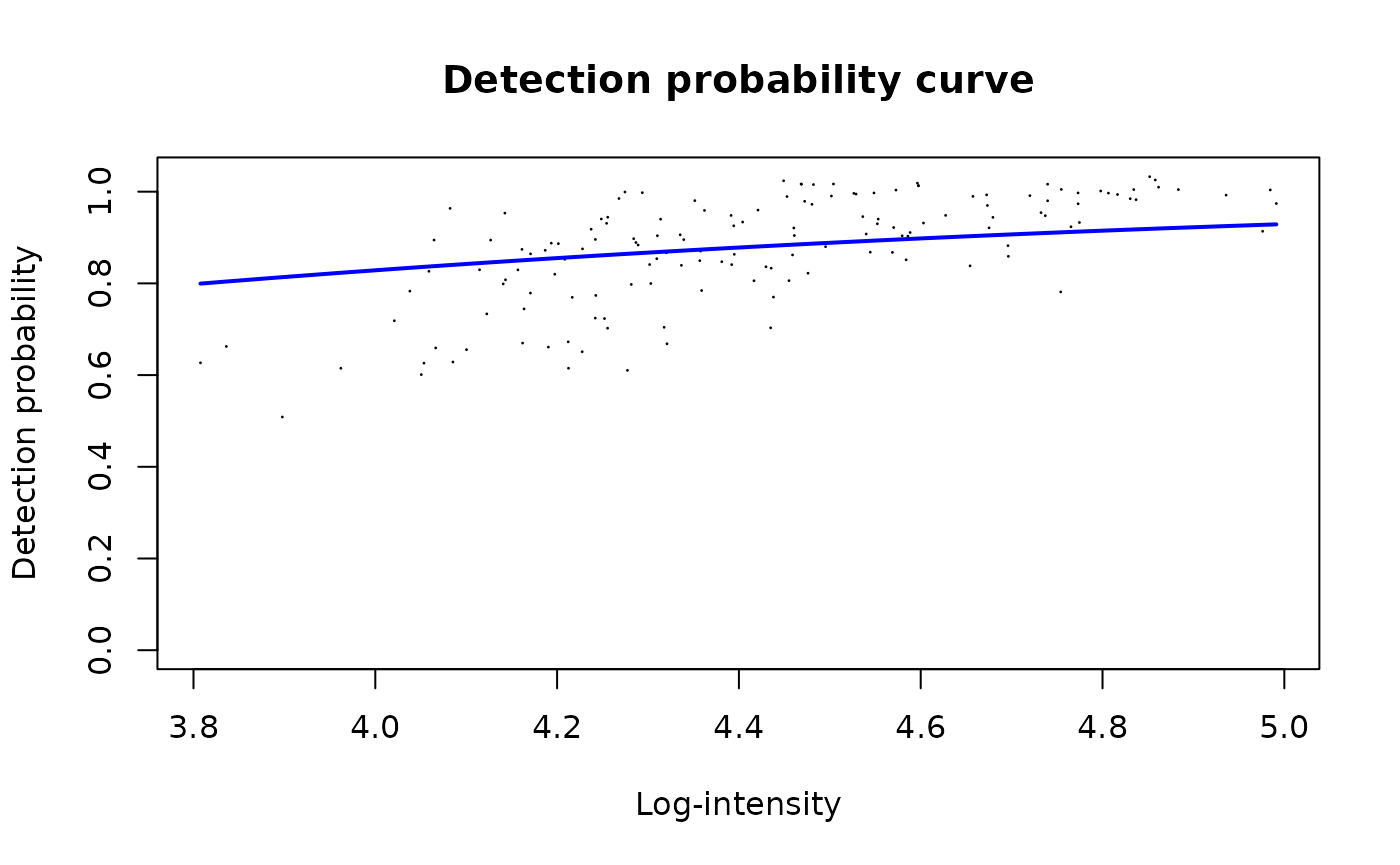

Example 1: Peptide-Level Analysis with limpa

Quantify peptides with `dpcQuantByRow()`

dpcQuantByRow() quantifies each peptide row independently (no protein aggregation). Internally it calls peptides2Proteins() with each row as its own “protein” (using protein.id = seq_len(nrow(y))). Missing values are not filled in with fabricated numbers — instead, Bayesian maximum posterior estimation integrates over the missing values using the DPC.

y_peptide <- limpa::dpcQuantByRow(expr_matrix, dpc = dpc_est)

The result is a limma EList object. Let’s inspect its structure:

cat("Class:", class(y_peptide), "\n")

## Class: EList

cat("Slots:", names(y_peptide), "\n\n")

## Slots: E genes other dpc

cat("$E — expression matrix (peptides x samples), no NAs:\n")

## $E — expression matrix (peptides x samples), no NAs:

cat("  dim:", dim(y_peptide$E), "\n")

##   dim: 152 15

cat("  NAs:", sum(is.na(y_peptide$E)), "\n")

##   NAs: 0

cat("  range:", round(range(y_peptide$E), 2), "\n\n")

##   range: 3.28 5.5

cat("$genes — per-peptide annotation:\n")

## $genes — per-peptide annotation:

str(y_peptide$genes)

## 'data.frame':    152 obs. of  1 variable:
##  $ PropObs: num  0.733 0.667 0.8 0.867 0.8 ...

cat("\n")

cat("$other — additional matrices:\n")

## $other — additional matrices:

cat("  names:", names(y_peptide$other), "\n")

##   names: n.observations standard.error

cat("  $n.observations — how many precursors were observed per row per sample:\n")

##   $n.observations — how many precursors were observed per row per sample:

cat("    range:", range(y_peptide$other$n.observations), "\n")

##     range: 0 1

cat("  $standard.error — posterior SD of the quantification:\n")

##   $standard.error — posterior SD of the quantification:

cat("    range:", round(range(y_peptide$other$standard.error), 4), "\n\n")

##     range: 0.01 0.3354

cat("$dpc — the DPC parameters used:\n")

## $dpc — the DPC parameters used:

print(y_peptide$dpc)

##     beta0     beta1 
## -2.424456  1.000000

Key fields:

$E: The quantified expression matrix. All NAs from the input have been replaced by maximum posterior estimates (integrating over the DPC). This is a complete matrix.
$other$standard.error: Per-peptide, per-sample posterior standard deviations. Peptides that were missing get larger SEs. This uncertainty is what limpa propagates into the DE model.
$other$n.observations: How many observations contributed (1 = observed, 0 = was missing).
$genes$PropObs: Proportion of samples where the peptide was observed.

Fit the DE model with `dpcDE()`

dpcDE() is a thin wrapper (9 lines of code) that calls voomaLmFitWithImputation(). Here is what it passes and why:

# From limpa/R/dpcDE.R:
dpcDE <- function(y, design, plot=TRUE, ...) {
  eps <- 1e-6
  voomaLmFitWithImputation(
    y         = y,                              # EList with $E and $other
    imputed   = !y$other$n.observations,        # logical matrix: TRUE where value was missing
    design    = design,                         # design matrix
    predictor = log(y$other$standard.error+eps),# log(SE) as precision predictor
    plot      = plot,
    ...
  )
}

Why vooma when SEs are already estimated?

The SEs from dpcQuantByRow()/dpcQuant() are per-observation quantification uncertainties. But limma needs observation-level precision weights for the linear model. voomaLmFitWithImputation() converts the SEs into proper weights via a bivariate lowess trend:

Fit an initial lmFit() to get per-protein residual SDs (sigma)
Model sqrt(sigma) ~ average_intensity + log(SE) using a bivariate linear predictor
Smooth with lowess to get a mean-variance trend function f()
Compute weights as w = 1/f(fitted_value)^4 — inverse fourth power of the predicted SD

This is analogous to how voom converts RNA-seq counts into weights via a mean-variance trend, but extended with a second predictor (the SE from quantification). The two predictors capture different variance sources:

Average intensity: the classical mean-variance relationship in proteomics
log(SE): additional variance from quantification uncertainty (more missing precursors = larger SE = lower weight)

Additionally, voomaLmFitWithImputation() corrects residual degrees of freedom for proteins where entire groups were missing (all values imputed), preventing overconfident inference.

fit_pep <- limpa::dpcDE(y_peptide, design, plot = TRUE)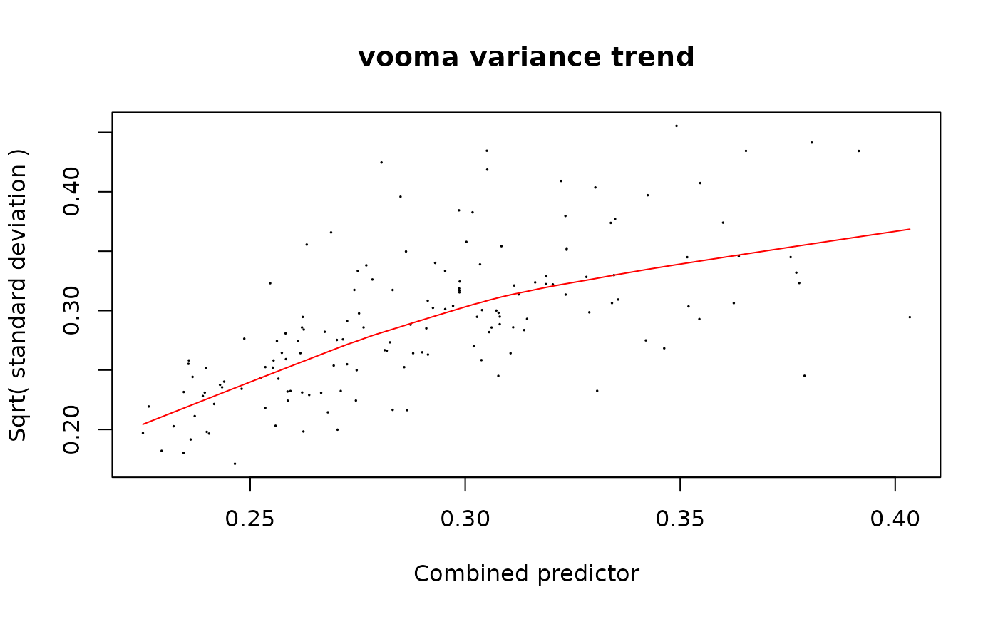

fit_pep <- limma::eBayes(fit_pep)

The plot shows sqrt(sigma) vs the combined predictor (average intensity + log SE). The red line is the lowess trend used to derive precision weights.

Test contrasts

fit_pep2 <- limma::contrasts.fit(fit_pep, cont_matrix)
fit_pep2 <- limma::eBayes(fit_pep2)

Results for A vs Ctrl at peptide level:

results_pep_A <- limma::topTable(fit_pep2, coef = "A_vs_Ctrl", number = 10, sort.by = "P")
print(results_pep_A)

##                                      PropObs      logFC  AveExpr         t
## 9VUkAq~8655~lfq~MuiCBcCu~lfq~light 1.0000000 -0.8851463 4.898474 -25.27012
## 7QuTub~5556~lfq~YmC8HPCi~lfq~light 0.8666667  0.9350267 4.727822  21.12259
## 9VUkAq~8655~lfq~JBvPc2qc~lfq~light 1.0000000  0.6970139 4.821333  20.11020
## 76k03k~9735~lfq~HZbAVyOK~lfq~light 1.0000000 -0.8821452 4.544532 -18.87531
## 9VUkAq~8655~lfq~SGFBeD1f~lfq~light 1.0000000  0.6462590 4.720641  18.42412
## ydeWJl~7145~lfq~39NMZpix~lfq~light 1.0000000  0.5177794 5.040518  17.54125
## JV3Z7t~7426~lfq~IpbWaJdN~lfq~light 0.9333333 -0.7605254 4.500164 -16.37530
## R2i6w7~5452~lfq~KFwoIdLY~lfq~light 0.8666667 -0.5710462 4.594583 -16.27149
## ZHBkZv~6720~lfq~eKM49i6K~lfq~light 1.0000000 -0.5051761 4.933688 -15.79546
## I1Jk2Z~7286~lfq~TKuvSqs3~lfq~light 0.8666667 -0.6480346 4.548221 -15.31439
##                                         P.Value    adj.P.Val        B
## 9VUkAq~8655~lfq~MuiCBcCu~lfq~light 2.474814e-24 3.761718e-22 45.50105
## 7QuTub~5556~lfq~YmC8HPCi~lfq~light 9.921774e-22 7.540549e-20 39.52930
## 9VUkAq~8655~lfq~JBvPc2qc~lfq~light 4.999951e-21 2.533308e-19 37.85792
## 76k03k~9735~lfq~HZbAVyOK~lfq~light 3.955088e-20 1.502933e-18 35.85932
## 9VUkAq~8655~lfq~SGFBeD1f~lfq~light 8.659287e-20 2.632423e-18 35.04942
## ydeWJl~7145~lfq~39NMZpix~lfq~light 4.202532e-19 1.064641e-17 33.32434
## JV3Z7t~7426~lfq~IpbWaJdN~lfq~light 3.740607e-18 8.122461e-17 31.31191
## R2i6w7~5452~lfq~KFwoIdLY~lfq~light 4.570919e-18 8.684746e-17 31.04096
## ZHBkZv~6720~lfq~eKM49i6K~lfq~light 1.160866e-17 1.960574e-16 30.03217
## I1Jk2Z~7286~lfq~TKuvSqs3~lfq~light 3.043369e-17 4.625921e-16 29.12106

Results for B vs Ctrl at peptide level:

results_pep_B <- limma::topTable(fit_pep2, coef = "B_vs_Ctrl", number = 10, sort.by = "P")
print(results_pep_B)

##                                      PropObs      logFC  AveExpr         t
## 9VUkAq~8655~lfq~40DK097A~lfq~light 0.9333333  1.0947462 4.809034  25.61456
## 9VUkAq~8655~lfq~MuiCBcCu~lfq~light 1.0000000 -0.6794121 4.898474 -21.57928
## MlNn1V~1396~lfq~PioauYsp~lfq~light 1.0000000 -0.6125184 4.818538 -18.95112
## I1Jk2Z~7286~lfq~TKuvSqs3~lfq~light 0.8666667 -0.8846547 4.548221 -17.11230
## 9VUkAq~8655~lfq~SGFBeD1f~lfq~light 1.0000000  0.5633911 4.720641  15.73300
## 7QuTub~5556~lfq~O5eT1xAS~lfq~light 1.0000000  0.6513203 4.574564  15.39969
## Fl4JiV~6934~lfq~tjP5Q817~lfq~light 0.8666667  0.5837830 4.719694  15.16521
## 7soopj~3451~lfq~WkbauTR1~lfq~light 1.0000000  0.4407287 4.899098  15.16147
## JcKVfU~1514~lfq~mCsMGaAU~lfq~light 1.0000000  0.6780110 4.330367  14.77820
## SGIVBl~4918~lfq~U6LlOS6x~lfq~light 0.8000000  0.8278659 4.200734  14.57807
##                                         P.Value    adj.P.Val        B
## 9VUkAq~8655~lfq~40DK097A~lfq~light 1.566024e-24 2.380356e-22 45.95730
## 9VUkAq~8655~lfq~MuiCBcCu~lfq~light 4.887857e-22 3.714772e-20 40.10657
## MlNn1V~1396~lfq~PioauYsp~lfq~light 3.472411e-20 1.759355e-18 35.84954
## I1Jk2Z~7286~lfq~TKuvSqs3~lfq~light 9.265355e-19 3.520835e-17 32.67289
## 9VUkAq~8655~lfq~SGFBeD1f~lfq~light 1.313960e-17 3.994439e-16 29.93253
## 7QuTub~5556~lfq~O5eT1xAS~lfq~light 2.561092e-17 6.488101e-16 29.18613
## Fl4JiV~6934~lfq~tjP5Q817~lfq~light 4.122372e-17 7.892554e-16 28.73952
## 7soopj~3451~lfq~WkbauTR1~lfq~light 4.153976e-17 7.892554e-16 28.59601
## JcKVfU~1514~lfq~mCsMGaAU~lfq~light 9.152959e-17 1.545833e-15 28.01480
## SGIVBl~4918~lfq~U6LlOS6x~lfq~light 1.390940e-16 2.114228e-15 27.68235

Summary of significant peptides (FDR < 0.05):

res_all_pep <- limma::topTable(fit_pep2, coef = "A_vs_Ctrl", number = Inf, sort.by = "none")
cat("A vs Ctrl: ", sum(res_all_pep$adj.P.Val < 0.05), "significant peptides at FDR < 0.05\n")

## A vs Ctrl:  122 significant peptides at FDR < 0.05

res_all_pep_B <- limma::topTable(fit_pep2, coef = "B_vs_Ctrl", number = Inf, sort.by = "none")
cat("B vs Ctrl: ", sum(res_all_pep_B$adj.P.Val < 0.05), "significant peptides at FDR < 0.05\n")

## B vs Ctrl:  115 significant peptides at FDR < 0.05

Low-Level API: Step-by-Step Peptide Analysis

This section decomposes the limpa pipeline into individual function calls, showing exactly what happens at each stage. We reuse the same expr_matrix, dpc_est, and design from above.

Step 1: Estimate the DPC

Already done above, but for completeness:

dpc_est <- limpa::dpc(expr_matrix)
cat("DPC: beta0 =", round(dpc_est$dpc["beta0"], 3),
    ", beta1 =", round(dpc_est$dpc["beta1"], 3), "\n")

## DPC: beta0 = -2.424 , beta1 = 1

The dpc() return value also contains hyperparameters estimated from the data:

cat("mu.prior  (prior mean of row means):", round(dpc_est$mu.prior, 3), "\n")

## mu.prior  (prior mean of row means): 4.448

cat("df.prior  (prior df for variance):", round(dpc_est$df.prior, 3), "\n")

## df.prior  (prior df for variance): 3.48

cat("s2.prior  (prior variance):", round(dpc_est$s2.prior, 3), "\n")

## s2.prior  (prior variance): 0.032

Step 2: Quantify peptides (row-level, no aggregation)

dpcQuantByRow() calls peptides2Proteins() internally, treating each row as its own “protein” (i.e., protein.id = 1:nrow(y)). The result is an EList:

y_pep <- limpa::dpcQuantByRow(expr_matrix, dpc = dpc_est)

Step 3: Prepare inputs for the variance model

dpcDE() is just 3 lines. Here we do what it does manually:

# Logical matrix: TRUE where the original value was missing
imputed_matrix <- !y_pep$other$n.observations

cat("Imputed values:", sum(imputed_matrix), "of", length(imputed_matrix), "\n")

## Imputed values: 278 of 2280

# Log(SE) as a precision predictor for the variance trend
eps <- 1e-6
predictor <- log(y_pep$other$standard.error + eps)

cat("Predictor (log SE) range:", round(range(predictor), 2), "\n")

## Predictor (log SE) range: -4.61 -1.09

Step 4: What `voomaLmFitWithImputation()` does internally

Below we manually replicate the internals of voomaLmFitWithImputation(). This is the core of limpa’s DE pipeline.

Step 4a: Initial linear model fit (unweighted)

First, fit a standard lmFit() without any precision weights. This gives per-peptide residual standard deviations (sigma) and fitted values.

fit0 <- limma::lmFit(y_pep, design)

cat("Initial fit — unweighted:\n")

## Initial fit — unweighted:

cat("  Coefficients:", dim(fit0$coefficients), "(peptides x groups)\n")

##   Coefficients: 152 3 (peptides x groups)

cat("  Sigma range:", round(range(fit0$sigma), 4), "\n")

##   Sigma range: 0.0293 0.2075

cat("  df.residual:", unique(fit0$df.residual), "\n")

##   df.residual: 12

# Compute per-observation fitted values (peptides x samples)
fitted_values <- fit0$coefficients %*% t(fit0$design)
cat("  Fitted values:", dim(fitted_values), "\n")

##   Fitted values: 152 15

Step 4b: DF correction for fully imputed groups

If a peptide has ALL values imputed within a design-matrix group, its fitted value for that group is determined entirely by imputed data — so the residual df should be reduced. This uses the hat matrix to detect such cases.

h <- 1 - hat(design)  # leverage complement per sample
df_imputed <- imputed_matrix %*% (1 - h)  # effective imputed df per peptide

n_affected <- sum(df_imputed > 0.9999)
cat("Peptides with fully-imputed groups:", n_affected, "\n")

## Peptides with fully-imputed groups: 16

# For affected peptides, refit on observed-only data to get corrected sigma/df
if (n_affected > 0) {
  affected_idx <- which(rowSums(df_imputed > 0.9999) > 0)
  E_affected <- y_pep$E[affected_idx, , drop = FALSE]
  E_affected_NA <- E_affected
  E_affected_NA[imputed_matrix[affected_idx, , drop = FALSE]] <- NA
  fit_NA <- suppressWarnings(limma::lmFit(E_affected_NA, design))

  cat("Corrected df.residual for affected peptides:", fit_NA$df.residual[1:min(5, length(fit_NA$df.residual))], "\n")

  # Replace sigma and df for affected rows
  fit0$sigma[affected_idx] <- fit_NA$sigma
  fit0$df.residual[affected_idx] <- fit_NA$df.residual
}

## Corrected df.residual for affected peptides: 7 7 6 7 6

Step 4c: Bivariate linear predictor (average intensity + log SE)

This is the key innovation over standard vooma. Instead of modelling variance as a function of average intensity alone, limpa uses TWO predictors:

sx = average log2 expression per peptide (classical mean-variance axis)
sxc = average log(SE) per peptide (quantification uncertainty axis)

A linear model sqrt(sigma) ~ sx + sxc combines them into a single predictor.

# Average expression per peptide
sx <- rowMeans(y_pep$E, na.rm = TRUE)

# Residual SD (square root for the variance trend)
sy <- sqrt(fit0$sigma)

# Average log(SE) per peptide — the precision predictor
sxc <- rowMeans(predictor, na.rm = TRUE)

# Bivariate linear model: sqrt(sigma) ~ 1 + avg_intensity + avg_log_SE
vartrend <- lm.fit(cbind(1, sx, sxc), sy)
beta <- coef(vartrend)
cat("Variance trend coefficients:\n")

## Variance trend coefficients:

cat("  Intercept:", round(beta[1], 4), "\n")

##   Intercept: 0.6832

cat("  avg_intensity:", round(beta[2], 4), "\n")

##   avg_intensity: -0.0789

cat("  avg_log_SE:", round(beta[3], 4),
    ifelse(beta[3] > 0, " (higher SE → higher variance, as expected)", ""), "\n")

##   avg_log_SE: 0.0119  (higher SE → higher variance, as expected)

# Combined predictor (per-peptide summary for the lowess x-axis)
sx_combined <- vartrend$fitted.values

# Per-observation combined predictor (for computing weights later)
mu_combined <- beta[1] + beta[2] * fitted_values + beta[3] * predictor

Step 4d: Lowess smoothing of the variance trend

Smooth the sqrt(sigma) ~ combined_predictor relationship with lowess. The smoothed trend function f() will be used to derive weights.

span <- limma::chooseLowessSpan(nrow(y_pep), small.n = 50, min.span = 0.3, power = 1/3)
cat("Lowess span:", round(span, 3), "\n")

## Lowess span: 0.783

l <- lowess(sx_combined, sy, f = span)

# Plot the trend
plot(sx_combined, sy,
     xlab = "Combined predictor (avg intensity + log SE)",
     ylab = "Sqrt(sigma)",
     pch = 16, cex = 0.5, col = "grey40",
     main = "vooma variance trend (manual)")
lines(l, col = "red", lwd = 2)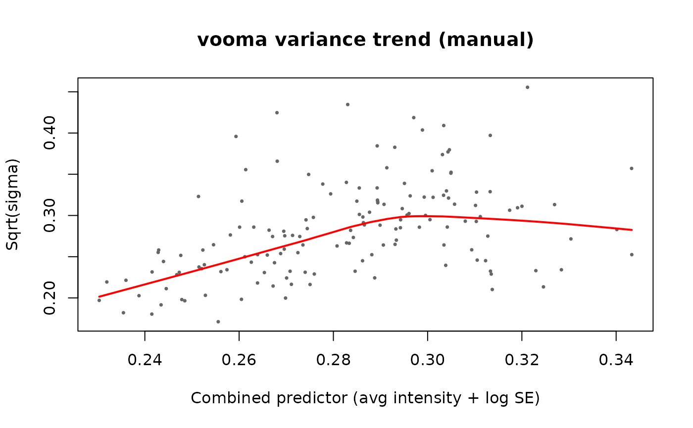

Step 4e: Derive precision weights

The lowess trend gives a function f() that predicts sqrt(sigma) from the combined predictor. Weights are the inverse fourth power: w = 1/f(mu)^4. This means observations with higher predicted variance get lower weight.

# Interpolating function from the lowess fit
f_trend <- approxfun(l, rule = 2, ties = list("ordered", mean))

# Per-observation weights: 1/f(mu_ij)^4
w_manual <- 1 / f_trend(mu_combined)^4
dim(w_manual) <- dim(y_pep$E)

cat("Weights matrix:", dim(w_manual), "\n")

## Weights matrix: 152 15

cat("Weight range:", round(range(w_manual), 2), "\n")

## Weight range: 124.89 606.68

cat("Weight median:", round(median(w_manual), 2), "\n")

## Weight median: 165.13

# Show how weights relate to missingness
cat("\nMean weight for observed values:", round(mean(w_manual[!imputed_matrix]), 2), "\n")

## 
## Mean weight for observed values: 237.64

cat("Mean weight for imputed values:", round(mean(w_manual[imputed_matrix]), 2), "\n")

## Mean weight for imputed values: 150.99

Imputed values get systematically lower weights because they have larger SEs, which pushes them to the high-variance end of the trend.

Step 4f: Final weighted linear model fit

Refit lmFit() using the vooma weights. This is the final model — coefficients now reflect precision-weighted estimates.

fit_vooma <- limma::lmFit(y_pep, design, weights = w_manual)

# Re-apply DF correction for affected peptides
if (n_affected > 0) {
  fit_NA_w <- suppressWarnings(limma::lmFit(E_affected_NA, design,
                                            weights = w_manual[affected_idx, , drop = FALSE]))
  fit_vooma$sigma[affected_idx] <- fit_NA_w$sigma
  fit_vooma$df.residual[affected_idx] <- fit_NA_w$df.residual
}

cat("Final weighted fit:\n")

## Final weighted fit:

cat("  Sigma range:", round(range(fit_vooma$sigma), 4), "\n")

##   Sigma range: 0.439 2.5172

cat("  df.residual range:", range(fit_vooma$df.residual), "\n")

##   df.residual range: 5 12

At this point fit_vooma is an MArrayLM with precision-weighted coefficient estimates but no empirical Bayes moderation yet.

Step 5: Empirical Bayes moderation with `eBayes()`

eBayes() shrinks the per-peptide variance estimates toward a common prior, producing moderated t-statistics with increased degrees of freedom:

fit_eb <- limma::eBayes(fit_vooma)

cat("Before eBayes — df.residual[1:5]:", fit_vooma$df.residual[1:5], "\n")

## Before eBayes — df.residual[1:5]: 12 7 12 12 12

cat("After eBayes  — df.total[1:5]:   ", fit_eb$df.total[1:5], "\n")

## After eBayes  — df.total[1:5]:    21.92524 16.92524 21.92524 21.92524 21.92524

cat("Prior df (df.prior):", round(fit_eb$df.prior, 2), "\n")

## Prior df (df.prior): 9.93

cat("Prior variance (s2.prior):", round(fit_eb$s2.prior, 4), "\n")

## Prior variance (s2.prior): 1.1021

Step 6: Compute contrasts with `contrasts.fit()`

contrasts.fit() re-parameterizes the fitted model from design-matrix coefficients to the contrasts of interest:

fit_contr <- limma::contrasts.fit(fit_eb, cont_matrix)
cat("Contrast coefficients:", colnames(fit_contr$coefficients), "\n")

## Contrast coefficients: A_vs_Ctrl B_vs_Ctrl

cat("Dimensions:", dim(fit_contr$coefficients), "\n")

## Dimensions: 152 2

Apply eBayes() again after re-parameterization (this re-computes moderated statistics for the contrast coefficients):

fit_contr <- limma::eBayes(fit_contr)

Step 7: Extract results with `topTable()`

tt_A <- limma::topTable(fit_contr, coef = "A_vs_Ctrl", number = 10, sort.by = "P")
print(tt_A)

##                                      PropObs      logFC  AveExpr         t
## 9VUkAq~8655~lfq~MuiCBcCu~lfq~light 1.0000000 -0.8851463 4.898474 -24.93390
## 9VUkAq~8655~lfq~JBvPc2qc~lfq~light 1.0000000  0.6970139 4.821333  20.12626
## 9VUkAq~8655~lfq~SGFBeD1f~lfq~light 1.0000000  0.6462590 4.720641  19.40684
## 76k03k~9735~lfq~HZbAVyOK~lfq~light 1.0000000 -0.8821452 4.544532 -18.90755
## ydeWJl~7145~lfq~39NMZpix~lfq~light 1.0000000  0.5177794 5.040518  18.22853
## 7QuTub~5556~lfq~YmC8HPCi~lfq~light 0.8666667  0.8763615 4.727822  17.92095
## ZHBkZv~6720~lfq~eKM49i6K~lfq~light 1.0000000 -0.5051761 4.933688 -16.46951
## R2i6w7~5452~lfq~KFwoIdLY~lfq~light 0.8666667 -0.5710462 4.594583 -16.12305
## R2i6w7~5452~lfq~2vAYUEfz~lfq~light 1.0000000  0.4678078 4.810543  15.99482
## ZHBkZv~6720~lfq~nLeEGNEy~lfq~light 1.0000000 -0.4166154 4.975519 -14.76092
##                                         P.Value    adj.P.Val        B
## 9VUkAq~8655~lfq~MuiCBcCu~lfq~light 1.392189e-17 2.116127e-15 30.41508
## 9VUkAq~8655~lfq~JBvPc2qc~lfq~light 1.261731e-15 9.589152e-14 25.86910
## 9VUkAq~8655~lfq~SGFBeD1f~lfq~light 2.690943e-15 1.363411e-13 25.16606
## 76k03k~9735~lfq~HZbAVyOK~lfq~light 4.620372e-15 1.755741e-13 24.63018
## ydeWJl~7145~lfq~39NMZpix~lfq~light 9.839263e-15 2.991136e-13 23.70404
## 7QuTub~5556~lfq~YmC8HPCi~lfq~light 1.397128e-14 3.539391e-13 23.49254
## ZHBkZv~6720~lfq~eKM49i6K~lfq~light 7.872433e-14 1.709443e-12 21.66616
## R2i6w7~5452~lfq~KFwoIdLY~lfq~light 1.212708e-13 2.304146e-12 21.30782
## R2i6w7~5452~lfq~2vAYUEfz~lfq~light 1.425879e-13 2.408151e-12 21.03298
## ZHBkZv~6720~lfq~nLeEGNEy~lfq~light 7.181412e-13 1.091575e-11 19.32675

topTable() returns:

logFC — the contrast estimate (log2 fold change)
AveExpr — average expression across all samples
t — moderated t-statistic
P.Value — p-value from the moderated t-test
adj.P.Val — BH-adjusted p-value (FDR)
B — log-odds of differential expression

Step 8: Verify equivalence with `dpcDE()` wrapper

The low-level pipeline should give identical results to dpcDE():

# Compare with the high-level result from Example 1
tt_highlevel <- limma::topTable(fit_pep2, coef = "A_vs_Ctrl", number = Inf, sort.by = "none")
tt_lowlevel <- limma::topTable(fit_contr, coef = "A_vs_Ctrl", number = Inf, sort.by = "none")

# Match by rownames and compare logFC
common <- intersect(rownames(tt_highlevel), rownames(tt_lowlevel))
max_diff <- max(abs(tt_highlevel[common, "logFC"] - tt_lowlevel[common, "logFC"]))
cat("Max logFC difference between high-level and low-level:", max_diff, "\n")

## Max logFC difference between high-level and low-level: 0.1740179

Example 2: Protein-Level Analysis with limpa

Quantify proteins with `dpcQuant()`

dpcQuant() aggregates peptides to proteins using Bayesian maximum posterior estimation. For each protein it fits an additive model: y_ij = mu_j + alpha_i + epsilon_ij where mu_j is the protein expression in sample j and alpha_i is the peptide-specific offset. Missing values are integrated out via the DPC (Gauss quadrature, 16 nodes).

protein_id <- rowdata$protein_Id
y_protein <- limpa::dpcQuant(expr_matrix, protein.id = protein_id, dpc = dpc_est)

Inspect the EList structure — same slots as peptide-level but now at protein level:

cat("Class:", class(y_protein), "\n")

## Class: EList

cat("Slots:", names(y_protein), "\n\n")

## Slots: E genes other dpc prior.mean prior.sd prior.logFC

cat("$E — protein expression matrix (no NAs):\n")

## $E — protein expression matrix (no NAs):

cat("  dim:", dim(y_protein$E), "\n")

##   dim: 50 15

cat("  NAs:", sum(is.na(y_protein$E)), "\n")

##   NAs: 0

cat("  range:", round(range(y_protein$E), 2), "\n\n")

##   range: 2.59 5.22

cat("$genes — per-protein annotation:\n")

## $genes — per-protein annotation:

str(y_protein$genes)

## 'data.frame':    50 obs. of  3 variables:
##  $ Protein  : chr  "0EfVhX~7161" "0m5WN4~3543" "76k03k~9735" "7cbcrd~0495" ...
##  $ NPeptides: num  4 1 3 2 12 2 7 1 1 1 ...
##  $ PropObs  : num  0.767 0.8 0.911 0.833 0.911 ...

cat("  NPrec: number of precursor peptides per protein\n")

##   NPrec: number of precursor peptides per protein

cat("  PropObs: proportion of (peptide x sample) values that were observed\n\n")

##   PropObs: proportion of (peptide x sample) values that were observed

cat("$other$standard.error — posterior SD of protein quantification:\n")

## $other$standard.error — posterior SD of protein quantification:

cat("  dim:", dim(y_protein$other$standard.error), "\n")

##   dim: 50 15

cat("  range:", round(range(y_protein$other$standard.error), 4), "\n")

##   range: 0.0544 0.9587

cat("  Proteins with more missing peptides get larger SEs.\n\n")

##   Proteins with more missing peptides get larger SEs.

cat("$other$n.observations — observed peptide count per protein x sample:\n")

## $other$n.observations — observed peptide count per protein x sample:

cat("  range:", range(y_protein$other$n.observations), "\n\n")

##   range: 0 13

cat("$dpc, $prior.mean, $prior.sd, $prior.logFC — hyperparameters:\n")

## $dpc, $prior.mean, $prior.sd, $prior.logFC — hyperparameters:

cat("  DPC:", round(y_protein$dpc, 3), "\n")

##   DPC: -2.424 1

cat("  prior.mean:", round(y_protein$prior.mean, 3), "\n")

##   prior.mean: 4.446

cat("  prior.sd:", round(y_protein$prior.sd, 3), "\n")

##   prior.sd: 1

cat("  prior.logFC:", round(y_protein$prior.logFC, 3), "\n")

##   prior.logFC: 1

Key difference from dpcQuantByRow(): Here multiple peptide rows are aggregated into one protein row. The $other$standard.error now reflects both the within-protein variance and the impact of missing peptides. $genes$NPrec records how many peptides each protein had.

Fit the DE model

Same dpcDE() call — it passes log(SE) as a precision predictor and the !n.observations matrix as the imputation indicator to voomaLmFitWithImputation().

fit_prot <- limpa::dpcDE(y_protein, design, plot = TRUE)

fit_prot <- limma::eBayes(fit_prot)

Test contrasts

fit_prot2 <- limma::contrasts.fit(fit_prot, cont_matrix)
fit_prot2 <- limma::eBayes(fit_prot2)

Results for A vs Ctrl at protein level:

results_prot_A <- limma::topTable(fit_prot2, coef = "A_vs_Ctrl", number = 10, sort.by = "P")
print(results_prot_A)

##                 Protein NPeptides   PropObs      logFC  AveExpr          t
## ZHBkZv~6720 ZHBkZv~6720         4 0.9833333 -0.2583529 4.950277 -14.812890
## WjJPCz~7827 WjJPCz~7827         1 1.0000000 -0.4403868 4.631240 -12.939813
## MlNn1V~1396 MlNn1V~1396         2 1.0000000 -0.2718993 4.821361 -12.855005
## HvIpHG~7584 HvIpHG~7584         5 0.9466667  0.2745891 4.514262  12.025025
## bzNYQZ~8203 bzNYQZ~8203         1 0.9333333  0.5416581 4.744370  11.055897
## 76k03k~9735 76k03k~9735         3 0.9111111 -0.4931572 4.421848 -10.758418
## HC8K98~2990 HC8K98~2990         5 0.8800000  0.3341429 4.294403  10.067536
## CGzoYe~1248 CGzoYe~1248         4 0.8500000 -0.4011100 4.332492  -9.800033
## RE5qEz~1673 RE5qEz~1673         1 0.9333333 -0.4840450 4.715879  -9.497032
## JV3Z7t~7426 JV3Z7t~7426         3 0.9555556 -0.3182202 4.405652  -9.425937
##                  P.Value    adj.P.Val         B
## ZHBkZv~6720 3.788107e-11 1.894053e-09 15.778245
## WjJPCz~7827 3.155911e-10 5.824345e-09 10.683672
## MlNn1V~1396 3.494607e-10 5.824345e-09 12.883890
## HvIpHG~7584 9.767647e-10 1.220956e-08 12.517331
## bzNYQZ~8203 3.494127e-09 3.494127e-08  7.619698
## 76k03k~9735 5.257879e-09 4.381566e-08  7.708104
## HC8K98~2990 1.405128e-08 1.003663e-07  9.583694
## CGzoYe~1248 2.083556e-08 1.302223e-07  7.423475
## RE5qEz~1673 3.286157e-08 1.825643e-07  6.098838
## JV3Z7t~7426 3.662376e-08 1.831188e-07  8.117291

Results for B vs Ctrl at protein level:

results_prot_B <- limma::topTable(fit_prot2, coef = "B_vs_Ctrl", number = 10, sort.by = "P")
print(results_prot_B)

##                 Protein NPeptides   PropObs      logFC  AveExpr          t
## bkh7dJ~8025 bkh7dJ~8025         8 0.8666667  0.2987677 4.294356  14.579753
## WjJPCz~7827 WjJPCz~7827         1 1.0000000 -0.5157402 4.631240 -13.799342
## 9VUkAq~8655 9VUkAq~8655         7 0.9809524  0.2236035 4.760002  13.643687
## GK8UnK~3043 GK8UnK~3043         3 0.8888889  0.4677256 4.510816  13.171632
## SGIVBl~4918 SGIVBl~4918         3 0.6666667  0.9271119 4.006036  12.388950
## ZDkJUz~5298 ZDkJUz~5298         2 0.9666667  0.4227250 4.777733  12.175197
## MlNn1V~1396 MlNn1V~1396         2 1.0000000 -0.2254504 4.821361 -11.338763
## aWq1bG~4505 aWq1bG~4505         1 1.0000000  0.3873877 4.879590  10.173520
## JV3Z7t~7426 JV3Z7t~7426         3 0.9555556 -0.3589473 4.405652  -9.932470
## r2J0Eh~3817 r2J0Eh~3817         1 0.9333333  0.5107426 4.557161   9.792109
##                  P.Value    adj.P.Val         B
## bkh7dJ~8025 4.868865e-11 2.304285e-09 15.529437
## WjJPCz~7827 1.157502e-10 2.304285e-09 14.746780
## 9VUkAq~8655 1.382571e-10 2.304285e-09 14.286364
## GK8UnK~3043 2.395066e-10 2.993833e-09 13.924139
## SGIVBl~4918 6.181167e-10 6.181167e-09 11.795752
## ZDkJUz~5298 8.076240e-10 6.730200e-09 12.826036
## MlNn1V~1396 2.387606e-09 1.705433e-08 11.463338
## aWq1bG~4505 1.204604e-08 7.528778e-08  9.900234
## JV3Z7t~7426 1.712711e-08 9.515063e-08  9.766882
## r2J0Eh~3817 2.108260e-08 1.054130e-07  9.631145

Summary of significant proteins (FDR < 0.05):

res_all_prot <- limma::topTable(fit_prot2, coef = "A_vs_Ctrl", number = Inf, sort.by = "none")
cat("limpa protein — A vs Ctrl: ", sum(res_all_prot$adj.P.Val < 0.05),
    "significant proteins at FDR < 0.05\n")

## limpa protein — A vs Ctrl:  41 significant proteins at FDR < 0.05

res_all_prot_B <- limma::topTable(fit_prot2, coef = "B_vs_Ctrl", number = Inf, sort.by = "none")
cat("limpa protein — B vs Ctrl: ", sum(res_all_prot_B$adj.P.Val < 0.05),
    "significant proteins at FDR < 0.05\n")

## limpa protein — B vs Ctrl:  39 significant proteins at FDR < 0.05

Summary Comparison

comparison <- data.frame(
  method = c("baseline limma (medpolish + lmFit)",
             "limpa peptide-level (dpcQuantByRow + dpcDE)",
             "limpa protein-level (dpcQuant + dpcDE)"),
  sig_A_vs_Ctrl = c(
    sum(results_baseline_A$adj.P.Val < 0.05),
    sum(res_all_pep$adj.P.Val < 0.05),
    sum(res_all_prot$adj.P.Val < 0.05)
  ),
  sig_B_vs_Ctrl = c(
    sum(results_baseline_B$adj.P.Val < 0.05),
    sum(res_all_pep_B$adj.P.Val < 0.05),
    sum(res_all_prot_B$adj.P.Val < 0.05)
  )
)
knitr::kable(comparison, col.names = c("Method", "Sig. A vs Ctrl", "Sig. B vs Ctrl"))

Method	Sig. A vs Ctrl	Sig. B vs Ctrl
baseline limma (medpolish + lmFit)	40	36
limpa peptide-level (dpcQuantByRow + dpcDE)	122	115
limpa protein-level (dpcQuant + dpcDE)	41	39

Key Takeaways

dpcQuantByRow() quantifies each peptide independently, returning an EList with $E (complete, no NAs), $other$standard.error (quantification uncertainty), and $other$n.observations (observation counts).
dpcQuant() additionally aggregates peptides to proteins, fitting a Bayesian additive model per protein. The EList gains $genes$NPrec (peptide counts) and hyperparameter fields ($dpc, $prior.mean, $prior.sd, $prior.logFC).
dpcDE() is a thin wrapper that calls voomaLmFitWithImputation() with:
- imputed = !y$other$n.observations — flags which values were missing
- predictor = log(y$other$standard.error) — SEs as a variance predictor
Why vooma on top of SEs? The SEs from dpcQuant() are per-observation quantification uncertainties. voomaLmFitWithImputation() uses them as a second predictor in a bivariate variance trend (sqrt(sigma) ~ avg_intensity + log(SE)) to derive observation-level precision weights w = 1/f(fitted)^4. This captures both the classical mean-variance relationship and the additional heteroscedasticity from missing values. It also corrects residual DF for proteins where entire groups were imputed.

Witold Wolski

2026-03-30

Setup and Data Simulation

Design Matrix and Contrasts

Baseline: Standard limma Analysis (no limpa)

Estimate the Detection Probability Curve (DPC)

Example 1: Peptide-Level Analysis with limpa

Quantify peptides with `dpcQuantByRow()`

Fit the DE model with `dpcDE()`

Test contrasts

Low-Level API: Step-by-Step Peptide Analysis

Step 1: Estimate the DPC

Step 2: Quantify peptides (row-level, no aggregation)

Step 3: Prepare inputs for the variance model

Step 4: What `voomaLmFitWithImputation()` does internally

Step 4a: Initial linear model fit (unweighted)

Step 4b: DF correction for fully imputed groups

Step 4c: Bivariate linear predictor (average intensity + log SE)

Step 4d: Lowess smoothing of the variance trend

Step 4e: Derive precision weights

Step 4f: Final weighted linear model fit

Step 5: Empirical Bayes moderation with `eBayes()`

Step 6: Compute contrasts with `contrasts.fit()`

Step 7: Extract results with `topTable()`

Step 8: Verify equivalence with `dpcDE()` wrapper

Example 2: Protein-Level Analysis with limpa

Quantify proteins with `dpcQuant()`

Fit the DE model

Test contrasts

Summary Comparison

Key Takeaways

Using limpa Directly on prolfqua Simulated Data

Witold Wolski

2026-03-30

Setup and Data Simulation

Design Matrix and Contrasts

Baseline: Standard limma Analysis (no limpa)

Estimate the Detection Probability Curve (DPC)

Example 1: Peptide-Level Analysis with limpa

Quantify peptides with dpcQuantByRow()

Fit the DE model with dpcDE()

Test contrasts

Low-Level API: Step-by-Step Peptide Analysis

Step 1: Estimate the DPC

Step 2: Quantify peptides (row-level, no aggregation)

Step 3: Prepare inputs for the variance model

Step 4: What voomaLmFitWithImputation() does internally

Step 4a: Initial linear model fit (unweighted)

Step 4b: DF correction for fully imputed groups

Step 4c: Bivariate linear predictor (average intensity + log SE)

Step 4d: Lowess smoothing of the variance trend

Step 4e: Derive precision weights

Step 4f: Final weighted linear model fit

Step 5: Empirical Bayes moderation with eBayes()

Step 6: Compute contrasts with contrasts.fit()

Step 7: Extract results with topTable()

Step 8: Verify equivalence with dpcDE() wrapper

Example 2: Protein-Level Analysis with limpa

Quantify proteins with dpcQuant()

Fit the DE model

Test contrasts

Summary Comparison

Key Takeaways

Quantify peptides with `dpcQuantByRow()`

Fit the DE model with `dpcDE()`

Step 4: What `voomaLmFitWithImputation()` does internally

Step 5: Empirical Bayes moderation with `eBayes()`

Step 6: Compute contrasts with `contrasts.fit()`

Step 7: Extract results with `topTable()`

Step 8: Verify equivalence with `dpcDE()` wrapper

Quantify proteins with `dpcQuant()`