DEqMS-style Count-Dependent Variance Moderation
Witold E. Wolski
2026-07-10
Source:vignettes/DEqMS_Moderation.Rmd
DEqMS_Moderation.RmdPurpose
This vignette demonstrates ContrastsModeratedDEqMS, a
count-dependent variance shrinkage method inspired by the DEqMS approach
(Zhu et al., 2020). It is a drop-in alternative to
ContrastsModerated:
-
ContrastsModerated(standard): applies a single global prior variance to all proteins — every protein is shrunk toward the same value. -
ContrastsModeratedDEqMS(count-dependent): the prior variance depends on the number of peptides/PSMs used to quantify each protein. Proteins quantified from many peptides get less shrinkage (their variance is already well estimated); proteins from few peptides get more.
This matters in proteomics because quantification depth varies hugely across proteins. A protein quantified from 20 peptides has a much better-estimated variance than one from 2 peptides, and they should not receive the same prior.
The user-facing API is identical to ContrastsModerated:
same downstream methods (get_contrasts,
get_Plotter, to_wide,
merge_contrasts_results).
How it works
-
Fit LOESS:
log(sigma^2) ~ log2(peptide_count)— captures the count-dependent variance trend. -
Estimate prior df (d0): from the residual variance
around the LOESS curve, using the
trigammaInverseapproach (same math as limma/squeezeVarRob). -
Count-specific prior variance:
s0^2(count)varies per protein, derived from the fitted LOESS curve. -
Posterior variance: Bayesian shrinkage combining
observed and prior:
var.post = (d0 * s0^2(count) + df * sigma^2) / (d0 + df) - Moderated t-statistics and p-values are recomputed with the posterior variance.
Data preparation
We use simulated protein-level data. The simulation includes a
nr_peptides column — the number of peptides per protein —
which is exactly the count we need.
library(prolfqua)
library(dplyr)
library(ggplot2)

istar <- sim_lfq_data_protein_config(Nprot = 200, weight_missing = 0.3)
lfqdata <- LFQData$new(istar$data, istar$config)
lfqdata$remove_small_intensities()

lt <- lfqdata$get_Transformer()
transformed <- lt$log2()$robscale()$lfq
transformed$rename_response("transformedIntensity")
Define contrasts
contr_spec <- c(
  "AvsCtrl" = "group_A - group_Ctrl",
  "BvsCtrl" = "group_B - group_Ctrl",
  "AvsB"    = "group_A - group_B"
)
Inspect peptide counts
At the low-level ContrastsModeratedDEqMS API we still
provide an explicit count table. The count column can be derived
directly from the LFQData object via
config$nr_children. In this simulated data set the count
variable is nr_peptides.
count_per_prot <- transformed$data_long() |>
  group_by(protein_Id) |>
  summarise(nr_peptides = max(.data[[transformed$nr_children_col()]], na.rm = TRUE))

ggplot(count_per_prot, aes(x = nr_peptides)) +
  geom_histogram(binwidth = 1, fill = "steelblue", color = "white") +
  labs(x = "Number of peptides per protein", y = "Count",
       title = "Distribution of peptide counts") +
  theme_minimal()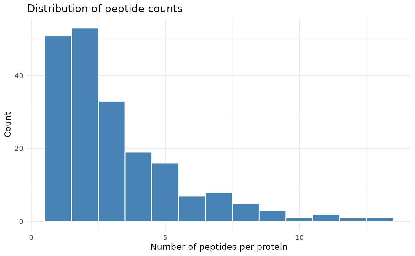
Standard moderation pipeline
mod_lm <- build_model(transformed, strategy_lm("transformedIntensity ~ group_"))
contr_lm <- prolfqua::Contrasts$new(mod_lm, contr_spec)
contr_moderated <- prolfqua::ContrastsModerated$new(contr_lm)
res_moderated <- contr_moderated$get_contrasts()
DEqMS moderation pipeline
The only difference: wrap with ContrastsModeratedDEqMS
instead of ContrastsModerated, and provide the
protein-level peptide counts. If you use the higher-level
build_contrast_analysis(..., method = "deqms") facade, that
count extraction is done for you from the LFQData
object.
contr_deqms <- ContrastsModeratedDEqMS$new(contr_lm, count_per_prot, "nr_peptides")
res_deqms <- contr_deqms$get_contrasts()
Diagnostic: variance vs. peptide count
This is the core diagnostic plot for the DEqMS approach. We expect
log(sigma^2) to decrease with increasing peptide count, and
the LOESS curve captures this trend.
# Get the unmoderated results with sigma and count
contr_raw <- contr_lm$get_contrasts()
contr_raw <- inner_join(
  contr_raw,
  count_per_prot,
  by = "protein_Id"
)

# Plot for one contrast
one_contrast <- contr_raw |> filter(contrast == levels(factor(contrast))[1])

ggplot(one_contrast, aes(x = log2(nr_peptides), y = log(sigma^2))) +
  geom_point(alpha = 0.4, size = 2) +
  geom_smooth(method = "loess", span = 0.75, color = "steelblue", se = TRUE) +
  labs(x = "log2(peptide count)",
       y = "log(residual variance)",
       title = paste("Variance vs. peptide count —", one_contrast$contrast[1])) +
  theme_minimal()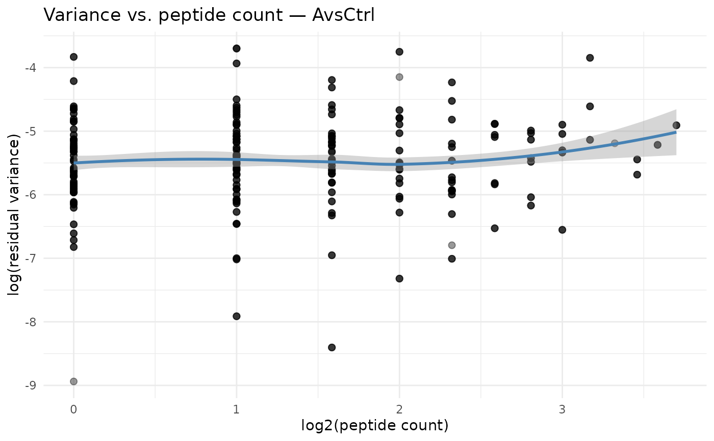
Residual variance decreases with peptide count. The LOESS curve (blue) defines the count-specific prior variance.
Comparing results
Fold changes are identical
Both decorators wrap the same underlying Contrasts
object, so fold changes are identical.
merged <- inner_join(
  select(res_deqms, protein_Id, contrast, diff_deqms = diff),
  select(res_moderated, protein_Id, contrast, diff_moderated = diff),
  by = c("protein_Id", "contrast")
)

cor(merged$diff_deqms, merged$diff_moderated, use = "complete.obs")
## [1] 1P-values differ (count-dependent shrinkage)
The DEqMS approach produces different p-values because the prior variance is protein-specific rather than global.
merged_p <- inner_join(
  select(res_deqms, protein_Id, contrast, p_deqms = p.value),
  select(res_moderated, protein_Id, contrast, p_moderated = p.value),
  by = c("protein_Id", "contrast")
)

cor(-log10(merged_p$p_deqms), -log10(merged_p$p_moderated), use = "complete.obs")
## [1] 0.9964816
ggplot(merged_p, aes(x = -log10(p_moderated), y = -log10(p_deqms))) +
  geom_point(alpha = 0.3, size = 1.5) +
  geom_abline(slope = 1, intercept = 0, color = "red", linetype = "dashed") +
  labs(x = "-log10(p) standard moderated",
       y = "-log10(p) DEqMS moderated") +
  theme_minimal()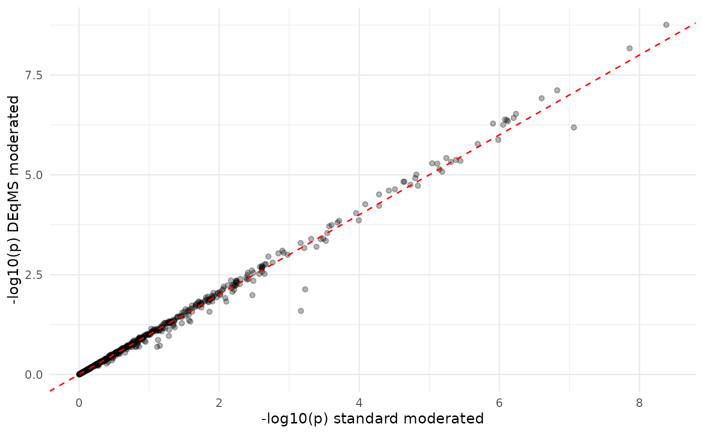
P-values: DEqMS vs. standard moderated. Highly correlated but not identical — DEqMS adjusts for peptide count.
Volcano plots
pl_moderated <- contr_moderated$get_Plotter()
pl_deqms <- contr_deqms$get_Plotter()

gridExtra::grid.arrange(
  pl_moderated$volcano()$FDR + ggtitle("Standard moderated"),
  pl_deqms$volcano()$FDR + ggtitle("DEqMS moderated"),
  ncol = 1
)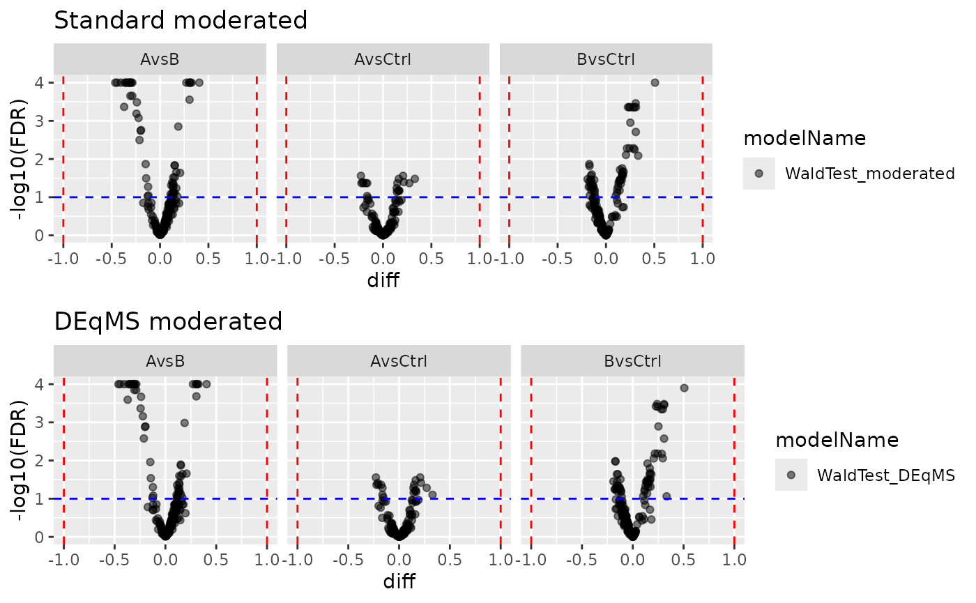
Volcano plots from both moderation approaches.
Merging with missing value imputation
ContrastsModeratedDEqMS works seamlessly with
ContrastsMissing and
merge_contrasts_results.
mC <- ContrastsMissing$new(lfqdata = transformed, contrasts = contr_spec)
merged_result <- merge_contrasts_results(prefer = contr_deqms, add = mC)

plotter <- merged_result$merged$get_Plotter()
plotter$volcano()$FDR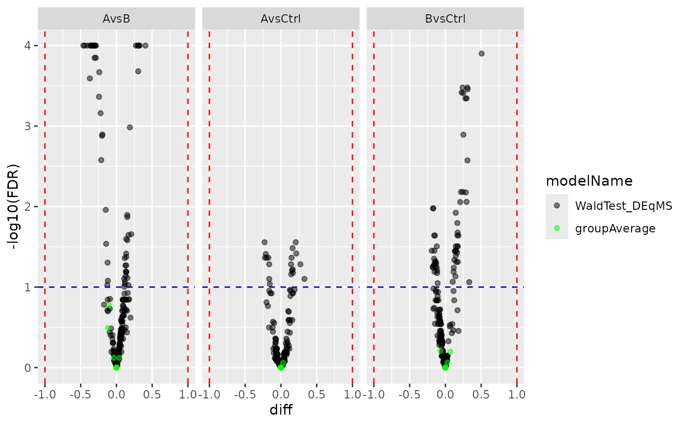
Wide format export
wide <- contr_deqms$to_wide()
head(wide)
## # A tibble: 6 × 13
## protein_Id diff.AvsCtrl diff.BvsCtrl diff.AvsB p.value.AvsCtrl p.value.BvsCtrl
## <chr> <dbl> <dbl> <dbl> <dbl> <dbl>
## 1 0EfVhX~76… 0.143 -0.128 0.272 0.00575 0.0117
## 2 0lCgkE~28… -0.0330 -0.000541 -0.0325 0.506 0.991
## 3 0m5WN4~11… 0.163 0.145 0.0182 0.000510 0.00111
## 4 0vgFfT~54… 0.0782 -0.0569 0.135 0.202 0.390
## 5 0YSKpy~75… -0.00621 -0.0244 0.0182 0.896 0.604
## 6 0ZHbvZ~41… 0.0471 -0.0402 0.0873 0.283 0.344
## # ℹ 7 more variables: p.value.AvsB <dbl>, FDR.AvsCtrl <dbl>, FDR.BvsCtrl <dbl>,
## # FDR.AvsB <dbl>, statistic.AvsCtrl <dbl>, statistic.BvsCtrl <dbl>,
## # statistic.AvsB <dbl>Inspecting all columns
Use all = TRUE to see both the original and moderated
columns side by side.
res_all <- contr_deqms$get_contrasts(all = TRUE)
res_all |>
  select(protein_Id, contrast, sigma, diff, statistic,
         moderated.var.prior, moderated.df.prior,
         moderated.var.post, moderated.statistic, moderated.p.value) |>
  head(10)
## # A tibble: 10 × 10
## protein_Id contrast sigma diff statistic moderated.var.prior
## <chr> <chr> <dbl> <dbl> <dbl> <dbl>
## 1 0EfVhX~7697 AvsCtrl 0.0659 0.143 3.07 0.00468
## 2 0lCgkE~2864 AvsCtrl 0.0531 -0.0330 -0.814 0.00459
## 3 0m5WN4~1168 AvsCtrl 0.0367 0.163 6.27 0.00444
## 4 0vgFfT~5498 AvsCtrl 0.0860 0.0782 1.29 0.00704
## 5 0YSKpy~7538 AvsCtrl 0.0632 -0.00621 -0.139 0.00468
## 6 0ZHbvZ~4125 AvsCtrl 0.0490 0.0471 1.36 0.00433
## 7 1HZ2jt~5236 AvsCtrl 0.0871 0.000509 0.00827 0.00474
## 8 3QLHfm~7883 AvsCtrl 0.116 -0.00875 -0.0756 0.00494
## 9 3QYop0~6494 AvsCtrl 0.0477 0.0796 2.04 0.00498
## 10 3Zhyy7~9324 AvsCtrl 0.0604 -0.0167 -0.338 0.00485
## # ℹ 4 more variables: moderated.df.prior <dbl>, moderated.var.post <dbl>,
## # moderated.statistic <dbl>, moderated.p.value <dbl>Note that moderated.var.prior varies per protein
(count-dependent), unlike in ContrastsModerated where it is
constant.
Session Info
## R version 4.5.2 (2025-10-31)
## Platform: x86_64-pc-linux-gnu
## Running under: Ubuntu 24.04.4 LTS
##
## Matrix products: default
## BLAS:   /usr/lib/x86_64-linux-gnu/openblas-pthread/libblas.so.3
## LAPACK: /usr/lib/x86_64-linux-gnu/openblas-pthread/libopenblasp-r0.3.26.so;  LAPACK version 3.12.0
##
## locale:
##  [1] LC_CTYPE=C.UTF-8       LC_NUMERIC=C           LC_TIME=C.UTF-8
##  [4] LC_COLLATE=C.UTF-8     LC_MONETARY=C.UTF-8    LC_MESSAGES=C.UTF-8
##  [7] LC_PAPER=C.UTF-8       LC_NAME=C              LC_ADDRESS=C
## [10] LC_TELEPHONE=C         LC_MEASUREMENT=C.UTF-8 LC_IDENTIFICATION=C
##
## time zone: UTC
## tzcode source: system (glibc)
##
## attached base packages:
## [1] stats     graphics  grDevices utils     datasets  methods   base
##
## other attached packages:
## [1] ggplot2_4.0.3  dplyr_1.2.1    prolfqua_1.6.3
##
## loaded via a namespace (and not attached):
##   [1] Rdpack_2.6.6           gridExtra_2.3.1        rlang_1.3.0
##   [4] magrittr_2.0.5         clue_0.3-68            GetoptLong_1.1.1
##   [7] otel_0.2.0             matrixStats_1.5.0      compiler_4.5.2
##  [10] mgcv_1.9-3             png_0.1-9              systemfonts_1.3.2
##  [13] vctrs_0.7.3            pkgconfig_2.0.3        shape_1.4.6.1
##  [16] crayon_1.5.3           fastmap_1.2.0          backports_1.5.1
##  [19] labeling_0.4.3         utf8_1.2.6             rmarkdown_2.31
##  [22] nloptr_2.2.1           ragg_1.5.2             UpSetR_1.4.1
##  [25] purrr_1.2.2            xfun_0.60              glmnet_5.0
##  [28] jomo_2.7-6             logistf_1.26.1         cachem_1.1.0
##  [31] jsonlite_2.0.0         progress_1.2.3         pan_2.0
##  [34] prettyunits_1.2.0      broom_1.0.13           parallel_4.5.2
##  [37] cluster_2.1.8.1        R6_2.6.1               bslib_0.11.0
##  [40] stringi_1.8.7          RColorBrewer_1.1-3     limma_3.66.0
##  [43] boot_1.3-32            rpart_4.1.24           jquerylib_0.1.4
##  [46] Rcpp_1.1.2             iterators_1.0.14       knitr_1.51
##  [49] IRanges_2.44.0         Matrix_1.7-4           splines_4.5.2
##  [52] nnet_7.3-20            tidyselect_1.2.1       yaml_2.3.12
##  [55] doParallel_1.0.17      codetools_0.2-20       lattice_0.22-7
##  [58] tibble_3.3.1           plyr_1.8.9             withr_3.0.3
##  [61] S7_0.2.2               evaluate_1.0.5         desc_1.4.3
##  [64] survival_3.8-3         circlize_0.4.18        pillar_1.11.1
##  [67] mice_3.19.0            foreach_1.5.2          stats4_4.5.2
##  [70] reformulas_0.4.4       plotly_4.12.0          generics_0.1.4
##  [73] S4Vectors_0.48.1       hms_1.1.4              scales_1.4.0
##  [76] minqa_1.2.8            glue_1.8.1             lazyeval_0.2.3
##  [79] tools_4.5.2            data.table_1.18.4      lme4_2.0-1
##  [82] forcats_1.0.1          fs_2.1.0               grid_4.5.2
##  [85] tidyr_1.3.2            rbibutils_2.4.1        colorspace_2.1-2
##  [88] nlme_3.1-168           formula.tools_1.7.1    cli_3.6.6
##  [91] textshaping_1.0.5      viridisLite_0.4.3      ComplexHeatmap_2.26.1
##  [94] gtable_0.3.6           sass_0.4.10            digest_0.6.39
##  [97] operator.tools_1.6.3.1 BiocGenerics_0.56.0    ggrepel_0.9.8
## [100] rjson_0.2.23           htmlwidgets_1.6.4      farver_2.1.2
## [103] htmltools_0.5.9        pkgdown_2.2.1          lifecycle_1.0.5
## [106] httr_1.4.8             GlobalOptions_0.1.4    mitml_0.4-5
## [109] statmod_1.5.2          MASS_7.3-65