Limma Backend for prolfqua

Purpose

This vignette demonstrates the limma backend for prolfqua’s modelling pipeline. The limma backend is a drop-in alternative to the per-protein lm + squeezeVar pipeline. Both approaches fit linear models and perform empirical Bayes variance shrinkage, but:

prolfqua default (strategy_lm + Contrasts + ContrastsModerated): fits one lm() per protein, then applies prolfqua’s own squeezeVarRob moderation.
limma backend (strategy_limma + ContrastsLimma): uses limma’s matrix-based lmFit + contrasts.fit + eBayes pipeline directly.

The user-facing API is identical: same formula specification, same contrast specification, same downstream methods (get_contrasts, get_Plotter, to_wide, merge_contrasts_results).

Data preparation

We use simulated protein-level data with 3 groups (A, B, Ctrl) and some missing values.

library(prolfqua)
library(dplyr)

istar <- sim_lfq_data_protein_config(Nprot = 100, weight_missing = 0.3)
lfqdata <- LFQData$new(istar$data, istar$config)
lfqdata$remove_small_intensities()

lt <- lfqdata$get_Transformer()
transformed <- lt$log2()$robscale()$lfq
transformed$rename_response("transformedIntensity")
transformed$factors()

## # A tibble: 12 × 3
##    sample  sampleName group_
##    <chr>   <chr>      <chr> 
##  1 A_V1    A_V1       A     
##  2 A_V2    A_V2       A     
##  3 A_V3    A_V3       A     
##  4 A_V4    A_V4       A     
##  5 B_V1    B_V1       B     
##  6 B_V2    B_V2       B     
##  7 B_V3    B_V3       B     
##  8 B_V4    B_V4       B     
##  9 Ctrl_V1 Ctrl_V1    Ctrl  
## 10 Ctrl_V2 Ctrl_V2    Ctrl  
## 11 Ctrl_V3 Ctrl_V3    Ctrl  
## 12 Ctrl_V4 Ctrl_V4    Ctrl

Define contrasts

The same contrast specification is used for both backends.

contr_spec <- c(
  "AvsCtrl" = "group_A - group_Ctrl",
  "BvsCtrl" = "group_B - group_Ctrl",
  "AvsB"    = "group_A - group_B"
)

prolfqua default pipeline

mod_lm <- build_model(transformed, strategy_lm("transformedIntensity ~ group_"))
contr_lm <- prolfqua::Contrasts$new(mod_lm, contr_spec)
contr_moderated <- ContrastsModerated$new(contr_lm)
res_moderated <- contr_moderated$get_contrasts()

Limma backend pipeline

The only difference is using strategy_limma + build_model_limma + ContrastsLimma.

strat_limma <- strategy_limma("transformedIntensity ~ group_")
mod_limma <- build_model_limma(transformed, strat_limma)
contr_limma <- ContrastsLimma$new(mod_limma, contr_spec)
res_limma <- contr_limma$get_contrasts()

Model-level inspection

The ModelLimma object supports the same inspection methods as Model.

mod_limma$get_anova() |> head()

## # A tibble: 6 × 5
##   protein_Id  F.value       p.value factor                     FDR
##   <chr>         <dbl>         <dbl> <chr>                    <dbl>
## 1 0EfVhX~3967  6.37   0.00377       group_B+group_Ctrl 0.0133     
## 2 0m5WN4~6025 28.8    0.00000000998 group_B+group_Ctrl 0.000000329
## 3 0YSKpy~2865  1.24   0.298         group_B+group_Ctrl 0.434      
## 4 3QLHfm~8938  7.57   0.00146       group_B+group_Ctrl 0.00805    
## 5 3QYop0~7543  0.0688 0.934         group_B+group_Ctrl 0.963      
## 6 76k03k~7094  3.12   0.0539        group_B+group_Ctrl 0.133

mod_limma$get_coefficients() |> head()

## # A tibble: 6 × 6
##   protein_Id  factor      Estimate Std..Error t.value Pr...t..
##   <chr>       <chr>          <dbl>      <dbl>   <dbl>    <dbl>
## 1 0EfVhX~3967 (Intercept)     4.47     0.0359    124. 6.83e-57
## 2 0m5WN4~6025 (Intercept)     4.10     0.0407    101. 6.81e-54
## 3 0YSKpy~2865 (Intercept)     4.16     0.0368    113. 4.05e-56
## 4 3QLHfm~8938 (Intercept)     4.55     0.0340    134. 2.07e-60
## 5 3QYop0~7543 (Intercept)     4.51     0.0350    129. 1.08e-59
## 6 76k03k~7094 (Intercept)     4.67     0.0355    132. 4.16e-60

mod_limma$anova_histogram()

## $plot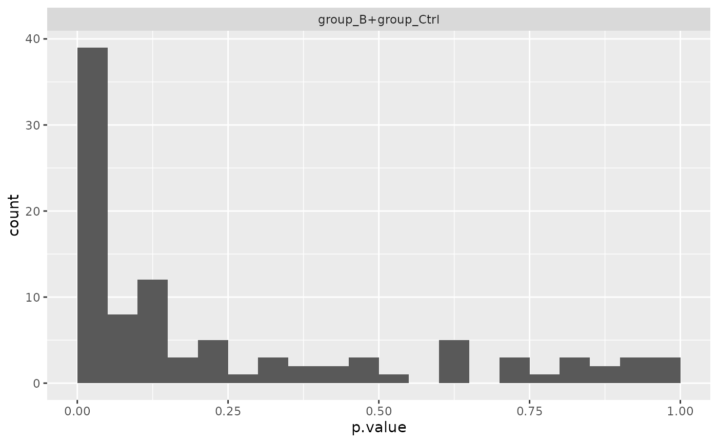

## 
## $name
## [1] "Anova_p.values_limma.pdf"

Comparing results

Fold changes are identical

Both backends estimate the same linear model, so fold changes (log2 FC) are identical.

merged <- inner_join(
  select(res_limma, protein_Id, contrast, diff_limma = diff),
  select(res_moderated, protein_Id, contrast, diff_moderated = diff),
  by = c("protein_Id", "contrast")
)

cor(merged$diff_limma, merged$diff_moderated, use = "complete.obs")

## [1] 1

plot(merged$diff_limma, merged$diff_moderated,
     xlab = "limma logFC", ylab = "prolfqua moderated logFC",
     pch = 20, col = rgb(0, 0, 0, 0.3))
abline(0, 1, col = "red")

Fold changes: limma vs. prolfqua moderated. Points lie on the diagonal.

P-values differ (different shrinkage)

The p-values differ because limma and prolfqua use different eBayes implementations, but they are highly correlated.

merged_p <- inner_join(
  select(res_limma, protein_Id, contrast, p_limma = p.value),
  select(res_moderated, protein_Id, contrast, p_moderated = p.value),
  by = c("protein_Id", "contrast")
)

cor(-log10(merged_p$p_limma), -log10(merged_p$p_moderated), use = "complete.obs")

## [1] 0.984774

plot(-log10(merged_p$p_limma), -log10(merged_p$p_moderated),
     xlab = "-log10(p) limma", ylab = "-log10(p) prolfqua moderated",
     pch = 20, col = rgb(0, 0, 0, 0.3))
abline(0, 1, col = "red")

P-values: limma vs. prolfqua moderated. High correlation but not identical.

Volcano plots

pl_limma <- contr_limma$get_Plotter()
pl_moderated <- contr_moderated$get_Plotter()

gridExtra::grid.arrange(
  pl_limma$volcano()$FDR + ggplot2::ggtitle("limma"),
  pl_moderated$volcano()$FDR + ggplot2::ggtitle("prolfqua moderated"),
  ncol = 1
)

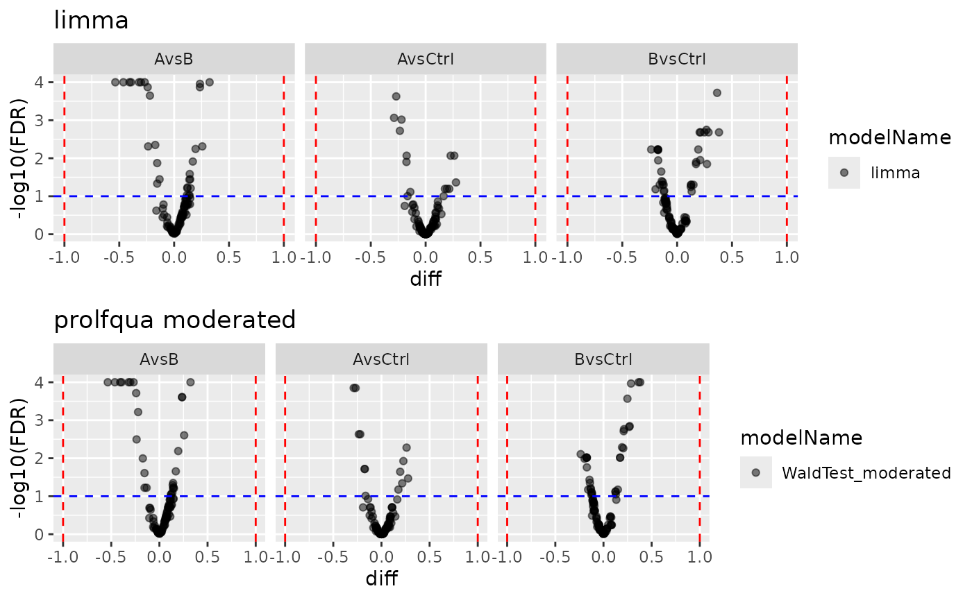
Volcano plots from both backends.

Merging with missing value imputation

ContrastsLimma integrates seamlessly with ContrastsMissing and merge_contrasts_results.

mC <- ContrastsMissing$new(lfqdata = transformed, contrasts = contr_spec)
merged_result <- merge_contrasts_results(prefer = contr_limma, add = mC)

plotter <- merged_result$merged$get_Plotter()
plotter$volcano()$FDR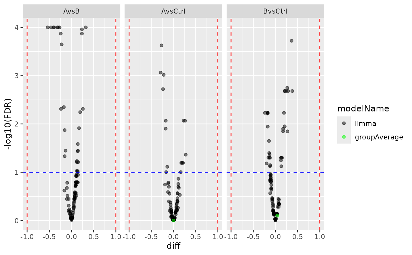

Wide format export

wide <- contr_limma$to_wide()
head(wide)

## # A tibble: 6 × 13
##   protein_Id diff.AvsCtrl diff.BvsCtrl diff.AvsB p.value.AvsCtrl p.value.BvsCtrl
##   <chr>             <dbl>        <dbl>     <dbl>           <dbl>           <dbl>
## 1 0EfVhX~39…      0.0875      -0.108      0.195        0.118            0.0555  
## 2 0m5WN4~60…     -0.235        0.172     -0.407        0.0000768        0.00258 
## 3 0YSKpy~28…      0.00148     -0.0703     0.0718       0.979            0.202   
## 4 3QLHfm~89…     -0.0343      -0.177      0.142        0.480            0.000641
## 5 3QYop0~75…     -0.0180      -0.00598   -0.0120       0.717            0.904   
## 6 76k03k~70…      0.0169      -0.0991     0.116        0.738            0.0544  
## # ℹ 7 more variables: p.value.AvsB <dbl>, FDR.AvsCtrl <dbl>, FDR.BvsCtrl <dbl>,
## #   FDR.AvsB <dbl>, statistic.AvsCtrl <dbl>, statistic.BvsCtrl <dbl>,
## #   statistic.AvsB <dbl>

Two-factor design

The limma backend handles multi-factor designs in the same way.

dd <- sim_lfq_data_2Factor_config(Nprot = 100, with_missing = FALSE)
lProt2 <- LFQData$new(dd$data, dd$config)
lProt2$rename_response("transformedIntensity")

strat2 <- strategy_limma("transformedIntensity ~ Treatment + Background")
mod2 <- build_model_limma(lProt2, strat2)

Contr2 <- c(
  "A_vs_B" = "TreatmentA - TreatmentB",
  "X_vs_Z" = "BackgroundX - BackgroundZ"
)
contr2 <- ContrastsLimma$new(mod2, Contr2)

pl2 <- contr2$get_Plotter()
pl2$volcano()$FDR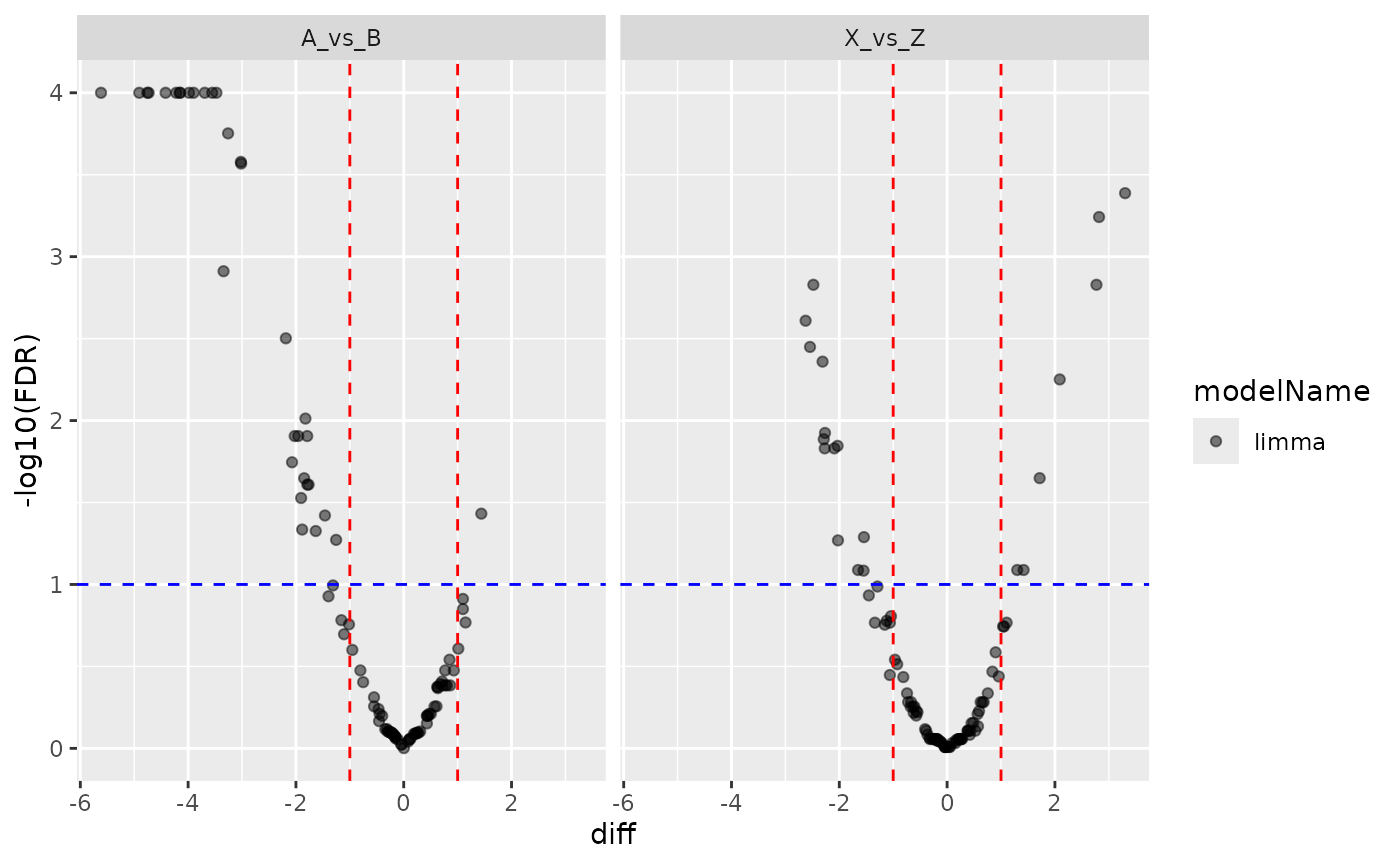

strategy_limma options

The strategy_limma function accepts trend and robust arguments that are passed to limma::eBayes:

trend = TRUE: allows the prior variance to depend on average intensity (useful when variance is intensity-dependent)
robust = TRUE: uses a robust empirical Bayes procedure (resistant to outlier variances)

strat_robust <- strategy_limma(
  "transformedIntensity ~ group_",
  trend = TRUE,
  robust = TRUE
)
mod_robust <- build_model_limma(transformed, strat_robust)
contr_robust <- ContrastsLimma$new(mod_robust, contr_spec)
head(contr_robust$get_contrasts())

## # A tibble: 6 × 13
##   modelName protein_Id  contrast     diff      FDR std.error statistic   p.value
##   <chr>     <chr>       <chr>       <dbl>    <dbl>     <dbl>     <dbl>     <dbl>
## 1 limma     0EfVhX~3967 AvsCtrl   0.0875  0.400       0.0551    1.59   0.113    
## 2 limma     0m5WN4~6025 AvsCtrl  -0.235   0.000672    0.0569   -4.13   0.0000408
## 3 limma     0YSKpy~2865 AvsCtrl   0.00148 0.992       0.0641    0.0230 0.982    
## 4 limma     3QLHfm~8938 AvsCtrl  -0.0343  0.778       0.0476   -0.721  0.471    
## 5 limma     3QYop0~7543 AvsCtrl  -0.0180  0.931       0.0475   -0.380  0.704    
## 6 limma     76k03k~7094 AvsCtrl   0.0169  0.931       0.0447    0.378  0.706    
## # ℹ 5 more variables: sigma <dbl>, df <dbl>, conf.low <dbl>, conf.high <dbl>,
## #   avgAbd <dbl>

Vooma backend pipeline

The vooma (variance modelling at the observational level) backend extends limma with observation-level precision weights derived from a mean-variance trend. This is analogous to voom for RNA-seq but applied to proteomics intensities. The key idea: instead of assuming equal variance across all observations, vooma estimates a smooth mean-variance relationship and down-weights observations with higher expected variance.

The API mirrors the standard limma pipeline — the only difference is calling build_model_limma_voom instead of build_model_limma.

strat_voom <- strategy_limma("transformedIntensity ~ group_")
mod_voom <- build_model_limma_voom(transformed, strat_voom, plot = TRUE)

contr_voom <- ContrastsLimma$new(mod_voom, contr_spec)
res_voom <- contr_voom$get_contrasts()

The plot shows sqrt(sigma) vs average log-expression. The red curve is the lowess trend used to derive per-observation weights.

Comparing limma vs vooma

merged_voom <- inner_join(
  select(res_limma, protein_Id, contrast, p_limma = p.value, diff_limma = diff),
  select(res_voom, protein_Id, contrast, p_voom = p.value, diff_voom = diff),
  by = c("protein_Id", "contrast")
)

data.frame(
  Metric = c("Fold-change correlation", "P-value correlation"),
  Value = c(
    cor(merged_voom$diff_limma, merged_voom$diff_voom, use = "complete.obs"),
    cor(-log10(merged_voom$p_limma), -log10(merged_voom$p_voom), use = "complete.obs")
  )
) |> knitr::kable(digits = 4)

Metric	Value
Fold-change correlation	1.0000
P-value correlation	0.9886

pl_voom <- contr_voom$get_Plotter()
gridExtra::grid.arrange(
  pl_limma$volcano()$FDR + ggplot2::ggtitle("limma"),
  pl_voom$volcano()$FDR + ggplot2::ggtitle("vooma"),
  ncol = 1
)

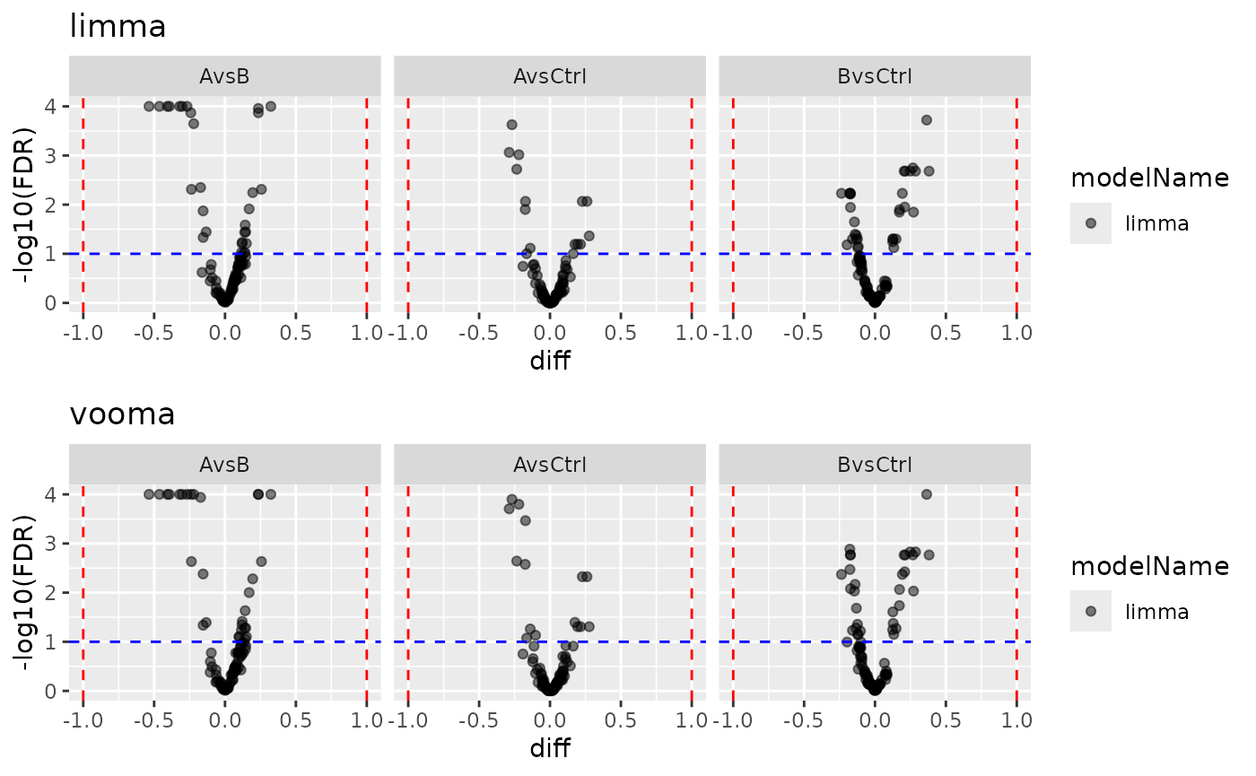
Volcano plots: limma vs vooma.

Limpa backend pipeline

The limpa backend uses limpa’s Detection Probability Curve (DPC) for probabilistic missing value handling, followed by vooma precision weighting that incorporates the quantification standard errors. The three-step pipeline is:

AggregateLimpa — estimates the DPC, then quantifies features using limpa::dpcQuant() (peptide→protein) or limpa::dpcQuantByRow() (same-level imputation). Produces standard errors and observation counts.
build_model_limpa — fits a vooma model using limpa::voomaLmFitWithImputation() with the SEs as a bivariate predictor
ContrastsLimma — reused as-is since the output is a standard MArrayLM

We show two examples: aggregation to protein level and staying at peptide level.

Prepare peptide-level data

Both examples start from the same simulated peptide-level dataset.

istar_pep <- sim_lfq_data_peptide_config(Nprot = 100)
lfq_peptide <- LFQData$new(istar_pep$data, istar_pep$config)
lfq_peptide <- lfq_peptide$get_Transformer()$log2()$lfq

data.frame(
  Property = c("Hierarchy", "Samples", "NAs"),
  Value = c(
    paste(lfq_peptide$config$hierarchy_keys(), collapse = " > "),
    length(unique(lfq_peptide$data[[lfq_peptide$config$sample_name]])),
    sum(is.na(lfq_peptide$data[[lfq_peptide$config$get_response()]]))
  )
) |> knitr::kable()

Property	Value
Hierarchy	protein_Id > peptide_Id
Samples	12
NAs	528

Example 1: Peptide → protein aggregation

Step 1: Aggregate with AggregateLimpa

AggregateLimpa wraps limpa::dpc() (DPC estimation) and limpa::dpcQuant() (protein quantification). The output is a protein-level LFQData with three value columns: intensity, standard error (config$opt_se), and observation count (config$nr_children). Missing values are probabilistically integrated out during quantification — no fabricated numbers are imputed.

agg <- AggregateLimpa$new(lfq_peptide, "protein")
lfq_protein_limpa <- agg$aggregate()

data.frame(
  Property = c("Input hierarchy", "Output hierarchy", "Response column",
               "SE column", "Nr children column", "NAs in output",
               "DPC beta0", "DPC beta1"),
  Value = c(
    paste(lfq_peptide$config$hierarchy_keys(), collapse = " > "),
    paste(lfq_protein_limpa$config$hierarchy_keys(), collapse = " > "),
    lfq_protein_limpa$config$get_response(),
    lfq_protein_limpa$config$opt_se,
    lfq_protein_limpa$config$nr_children,
    sum(is.na(lfq_protein_limpa$data[[lfq_protein_limpa$config$get_response()]])),
    round(agg$dpc_result$dpc[1], 3),
    round(agg$dpc_result$dpc[2], 3)
  )
) |> knitr::kable()

Property	Value
Input hierarchy	protein_Id > peptide_Id
Output hierarchy	protein_Id
Response column	limpa
SE column	limpa_se
Nr children column	nr_children_protein_Id
NAs in output	0
DPC beta0	-2.372
DPC beta1	1

Step 2: Build model with build_model_limpa

build_model_limpa extracts the SE and observation count matrices from the aggregated data and passes them to limpa::voomaLmFitWithImputation(). The SEs serve as a second predictor in the vooma variance trend (bivariate: average intensity + log SE), and the observation counts identify imputed entries for degree-of-freedom correction.

response <- lfq_protein_limpa$config$get_response()
strat_limpa <- strategy_limpa(paste(response, "~ group_"), plot = TRUE)
mod_limpa_prot <- build_model_limpa(lfq_protein_limpa, strat_limpa)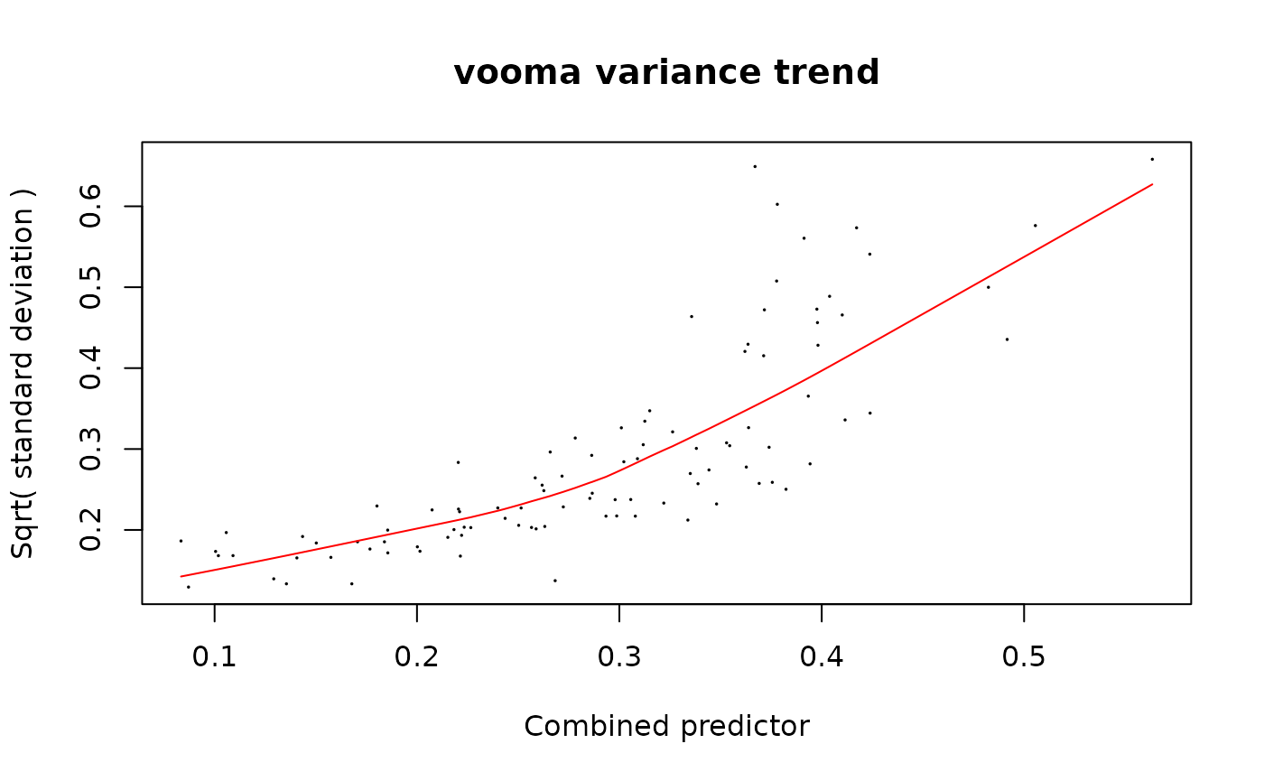

data.frame(
  Property = c("Model class", "Model name"),
  Value = c(class(mod_limpa_prot)[1], mod_limpa_prot$modelName)
) |> knitr::kable()

Property	Value
Model class	ModelLimma
Model name	limpa

mod_limpa_prot$get_coefficients() |> head() |> knitr::kable(digits = 3)

protein_Id	factor	Estimate	Std..Error	t.value
0EfVhX~3967	(Intercept)	4.566	0.032	140.675
0m5WN4~6025	(Intercept)	4.270	0.022	196.778
0YSKpy~2865	(Intercept)	4.061	0.048	85.005
3QLHfm~8938	(Intercept)	4.652	0.034	135.632
3QYop0~7543	(Intercept)	4.564	0.014	331.068
76k03k~7094	(Intercept)	4.539	0.014	314.082

Step 3: Compute contrasts with ContrastsLimma

Since build_model_limpa returns a standard ModelLimma, we reuse ContrastsLimma directly — same as for the limma and vooma backends.

contr_limpa_prot <- ContrastsLimma$new(mod_limpa_prot, contr_spec, modelName = "limpa")
res_limpa_prot <- contr_limpa_prot$get_contrasts()
head(res_limpa_prot) |> knitr::kable(digits = 3)

modelName	protein_Id	contrast	diff	FDR	std.error	statistic	p.value	sigma	df	conf.low	conf.high	avgAbd
limpa	0EfVhX~3967	AvsCtrl	0.188	0.005	0.056	3.353	0.002	0.772	25.515	0.073	0.303	4.472
limpa	0m5WN4~6025	AvsCtrl	0.078	0.033	0.032	2.418	0.023	0.855	25.515	0.012	0.145	4.231
limpa	0YSKpy~2865	AvsCtrl	-0.125	0.059	0.059	-2.108	0.045	0.968	25.515	-0.247	-0.003	4.124
limpa	3QLHfm~8938	AvsCtrl	0.233	0.011	0.080	2.929	0.007	0.927	25.515	0.069	0.397	4.535
limpa	3QYop0~7543	AvsCtrl	-0.133	0.000	0.018	-7.379	0.000	0.887	25.515	-0.170	-0.096	4.630
limpa	76k03k~7094	AvsCtrl	-0.112	0.000	0.019	-5.814	0.000	0.966	25.515	-0.151	-0.072	4.595

Volcano plot

pl_limpa_prot <- contr_limpa_prot$get_Plotter()
pl_limpa_prot$volcano()$FDR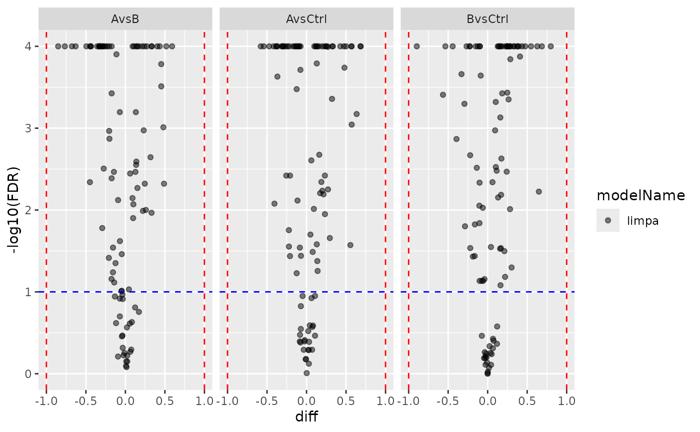

Limpa protein-level volcano plot.

Facade shortcut

The same pipeline is available as a one-liner via build_contrast_analysis(method = "limpa"). The input must be AggregateLimpa output (not plain get_Aggregator() output), because the facade needs the SE and observation count columns.

fa_limpa_prot <- build_contrast_analysis(
  lfq_protein_limpa, "~ group_", contr_spec, method = "limpa"
)
fa_limpa_prot$get_contrasts() |> head() |> knitr::kable(digits = 3)

facade	modelName	protein_Id	contrast	diff	FDR	std.error	statistic	p.value	sigma	df	conf.low	conf.high	avgAbd
limpa	limpa	0EfVhX~3967	AvsCtrl	0.188	0.005	0.056	3.353	0.002	0.772	25.515	0.073	0.303	4.472
limpa	limpa	0m5WN4~6025	AvsCtrl	0.078	0.033	0.032	2.418	0.023	0.855	25.515	0.012	0.145	4.231
limpa	limpa	0YSKpy~2865	AvsCtrl	-0.125	0.059	0.059	-2.108	0.045	0.968	25.515	-0.247	-0.003	4.124
limpa	limpa	3QLHfm~8938	AvsCtrl	0.233	0.011	0.080	2.929	0.007	0.927	25.515	0.069	0.397	4.535
limpa	limpa	3QYop0~7543	AvsCtrl	-0.133	0.000	0.018	-7.379	0.000	0.887	25.515	-0.170	-0.096	4.630
limpa	limpa	76k03k~7094	AvsCtrl	-0.112	0.000	0.019	-5.814	0.000	0.966	25.515	-0.151	-0.072	4.595

Example 2: Peptide-level analysis (no aggregation)

In this example we stay at the peptide level. AggregateLimpa with impute_only = TRUE calls limpa::dpcQuantByRow(), which fills in missing values at the peptide level while preserving the full hierarchy. Each peptide row is treated as its own “protein” (one peptide per group). The output has the same hierarchy as the input but with no NAs and with SE and observation count columns attached.

This is useful for peptidoform-level analyses (e.g. PTMs) where aggregation to protein level is not desired.

Step 1: Impute at peptide level

agg_pep <- AggregateLimpa$new(lfq_peptide, impute_only = TRUE)
lfq_peptide_limpa <- agg_pep$aggregate()

data.frame(
  Property = c("Input hierarchy", "Output hierarchy",
               "NAs in input", "NAs in output", "SE column"),
  Value = c(
    paste(lfq_peptide$config$hierarchy_keys(), collapse = " > "),
    paste(lfq_peptide_limpa$config$hierarchy_keys(), collapse = " > "),
    sum(is.na(lfq_peptide$data[[lfq_peptide$config$get_response()]])),
    sum(is.na(lfq_peptide_limpa$data[[lfq_peptide_limpa$config$get_response()]])),
    lfq_peptide_limpa$config$opt_se
  )
) |> knitr::kable()

Property	Value
Input hierarchy	protein_Id > peptide_Id
Output hierarchy	protein_Id > peptide_Id
NAs in input	528
NAs in output	0
SE column	limpa_se

Step 2: Build model at peptide level

The peptide-level data still has protein_Id and peptide_Id in its hierarchy. We set hierarchyDepth so that hierarchy_keys() returns only protein_Id — this makes the data “aggregated” from the model’s perspective (one row per protein_Id × peptide_Id × sample, with subject_Id = protein_Id).

Since each peptide is a separate row in the wide matrix, build_model_limpa fits the model at the peptide level.

response_pep <- lfq_peptide_limpa$config$get_response()
strat_limpa_pep <- strategy_limpa(paste(response_pep, "~ group_"), plot = TRUE)
mod_limpa_pep <- build_model_limpa(lfq_peptide_limpa, strat_limpa_pep)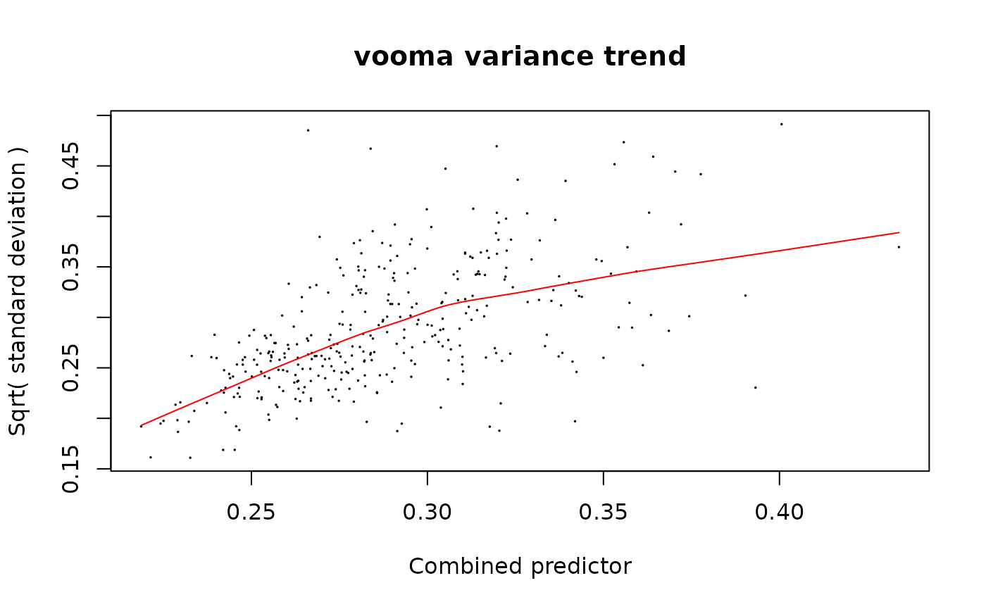

data.frame(
  Property = c("Model class", "Rows in model (peptides)"),
  Value = c(class(mod_limpa_pep)[1], nrow(mod_limpa_pep$fit$coefficients))
) |> knitr::kable()

Property	Value
Model class	ModelLimma
Rows in model (peptides)	350

Step 3: Compute contrasts

contr_limpa_pep <- ContrastsLimma$new(mod_limpa_pep, contr_spec, modelName = "limpa_peptide")
res_limpa_pep <- contr_limpa_pep$get_contrasts()

data.frame(
  Property = c("Peptide-level results", "Unique peptides"),
  Value = c(nrow(res_limpa_pep), length(unique(res_limpa_pep$peptide_Id)))
) |> knitr::kable()

Property	Value
Peptide-level results	1050
Unique peptides	350

head(res_limpa_pep) |> knitr::kable(digits = 3)

modelName	protein_Id	peptide_Id	contrast	diff	FDR	std.error	statistic	p.value	sigma	df	conf.low	conf.high	avgAbd
limpa_peptide	0EfVhX~3967	IIhYJDAe	AvsCtrl	0.234	0.000	0.046	5.086	0.000	1.047	35.777	0.141	0.327	4.545
limpa_peptide	0EfVhX~3967	SWkbauTR	AvsCtrl	0.156	0.021	0.061	2.562	0.015	1.208	35.777	0.033	0.280	4.393
limpa_peptide	0m5WN4~6025	7uKIY8WX	AvsCtrl	-0.430	0.000	0.067	-6.396	0.000	1.164	35.777	-0.566	-0.293	4.041
limpa_peptide	0m5WN4~6025	7xDNA2B6	AvsCtrl	0.272	0.000	0.061	4.485	0.000	1.069	35.777	0.149	0.395	4.187
limpa_peptide	0m5WN4~6025	KT0ROM7b	AvsCtrl	0.697	0.000	0.058	11.988	0.000	1.071	35.777	0.579	0.815	4.186
limpa_peptide	0m5WN4~6025	LYLauRlr	AvsCtrl	-0.413	0.000	0.049	-8.470	0.000	1.108	35.777	-0.512	-0.314	4.553

Volcano plot

pl_limpa_pep <- contr_limpa_pep$get_Plotter()
pl_limpa_pep$volcano()$FDR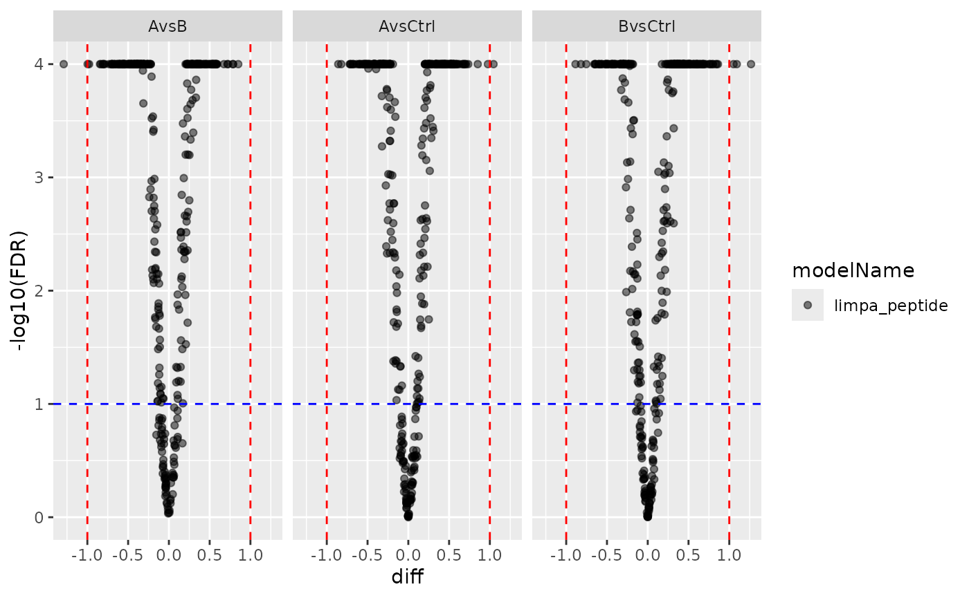

Limpa peptide-level volcano plot.

Comparison: protein-level vs peptide-level limpa

data.frame(
  Level = c("Protein", "Peptide"),
  Rows = c(nrow(res_limpa_prot), nrow(res_limpa_pep)),
  Proteins = c(length(unique(res_limpa_prot$protein_Id)),
               length(unique(res_limpa_pep$protein_Id))),
  Peptides = c(NA_integer_, length(unique(res_limpa_pep$peptide_Id)))
) |> knitr::kable()

Level	Rows	Proteins	Peptides
Protein	300	100	NA
Peptide	1050	100	350

Session Info

sessionInfo()

## R version 4.5.2 (2025-10-31)
## Platform: x86_64-pc-linux-gnu
## Running under: Ubuntu 24.04.4 LTS
## 
## Matrix products: default
## BLAS:   /usr/lib/x86_64-linux-gnu/openblas-pthread/libblas.so.3 
## LAPACK: /usr/lib/x86_64-linux-gnu/openblas-pthread/libopenblasp-r0.3.26.so;  LAPACK version 3.12.0
## 
## locale:
##  [1] LC_CTYPE=C.UTF-8       LC_NUMERIC=C           LC_TIME=C.UTF-8       
##  [4] LC_COLLATE=C.UTF-8     LC_MONETARY=C.UTF-8    LC_MESSAGES=C.UTF-8   
##  [7] LC_PAPER=C.UTF-8       LC_NAME=C              LC_ADDRESS=C          
## [10] LC_TELEPHONE=C         LC_MEASUREMENT=C.UTF-8 LC_IDENTIFICATION=C   
## 
## time zone: UTC
## tzcode source: system (glibc)
## 
## attached base packages:
## [1] stats     graphics  grDevices utils     datasets  methods   base     
## 
## other attached packages:
## [1] dplyr_1.2.0    prolfqua_1.6.1
## 
## loaded via a namespace (and not attached):
##  [1] tidyselect_1.2.1       viridisLite_0.4.3      farver_2.1.2          
##  [4] S7_0.2.1               fastmap_1.2.0          lazyeval_0.2.2        
##  [7] digest_0.6.39          rpart_4.1.24           lifecycle_1.0.5       
## [10] survival_3.8-3         statmod_1.5.1          magrittr_2.0.4        
## [13] compiler_4.5.2         progress_1.2.3         rlang_1.1.7           
## [16] sass_0.4.10            tools_4.5.2            utf8_1.2.6            
## [19] yaml_2.3.12            data.table_1.18.2.1    limpa_1.2.5           
## [22] knitr_1.51             labeling_0.4.3         prettyunits_1.2.0     
## [25] htmlwidgets_1.6.4      plyr_1.8.9             RColorBrewer_1.1-3    
## [28] withr_3.0.2            purrr_1.2.1            desc_1.4.3            
## [31] nnet_7.3-20            grid_4.5.2             jomo_2.7-6            
## [34] mice_3.19.0            ggplot2_4.0.2          scales_1.4.0          
## [37] iterators_1.0.14       MASS_7.3-65            cli_3.6.5             
## [40] crayon_1.5.3           UpSetR_1.4.0           rmarkdown_2.31        
## [43] ragg_1.5.2             reformulas_0.4.4       generics_0.1.4        
## [46] otel_0.2.0             httr_1.4.8             minqa_1.2.8           
## [49] cachem_1.1.0           operator.tools_1.6.3.1 splines_4.5.2         
## [52] vctrs_0.7.2            boot_1.3-32            glmnet_4.1-10         
## [55] Matrix_1.7-4           jsonlite_2.0.0         hms_1.1.4             
## [58] mitml_0.4-5            ggrepel_0.9.8          systemfonts_1.3.2     
## [61] foreach_1.5.2          limma_3.66.0           plotly_4.12.0         
## [64] tidyr_1.3.2            jquerylib_0.1.4        glue_1.8.0            
## [67] pkgdown_2.2.0          nloptr_2.2.1           pan_1.9               
## [70] codetools_0.2-20       stringi_1.8.7          shape_1.4.6.1         
## [73] gtable_0.3.6           lme4_2.0-1             tibble_3.3.1          
## [76] pillar_1.11.1          htmltools_0.5.9        R6_2.6.1              
## [79] textshaping_1.0.5      Rdpack_2.6.6           formula.tools_1.7.1   
## [82] evaluate_1.0.5         lattice_0.22-7         rbibutils_2.4.1       
## [85] backports_1.5.0        pheatmap_1.0.13        broom_1.0.12          
## [88] bslib_0.10.0           Rcpp_1.1.1             gridExtra_2.3         
## [91] nlme_3.1-168           mgcv_1.9-3             logistf_1.26.1        
## [94] xfun_0.57              fs_2.0.1               forcats_1.0.1         
## [97] pkgconfig_2.0.3

Witold E. Wolski

2026-04-02

Purpose

Data preparation

Define contrasts

prolfqua default pipeline

Limma backend pipeline

Model-level inspection

Comparing results

Fold changes are identical

P-values differ (different shrinkage)

Volcano plots

Merging with missing value imputation

Wide format export

Two-factor design

strategy_limma options

Vooma backend pipeline

Comparing limma vs vooma

Limpa backend pipeline

Prepare peptide-level data

Example 1: Peptide → protein aggregation

Step 1: Aggregate with AggregateLimpa

Step 2: Build model with build_model_limpa

Step 3: Compute contrasts with ContrastsLimma

Volcano plot

Facade shortcut

Example 2: Peptide-level analysis (no aggregation)

Step 1: Impute at peptide level

Step 2: Build model at peptide level

Step 3: Compute contrasts

Volcano plot

Comparison: protein-level vs peptide-level limpa

Session Info